4 Coordinate systems
In the last chapter, we discussed points and vectors and said that these geometrical concepts are crucial to specifying shapes of objects in virtual scenes. However, there is one big problem: we do not know how to represent these concepts in a computer. If we cannot do so, we would not be able to get a computer to do calculations on the shapes. We would not be able to render them and display them to any users, and there would be no computer graphics! This chapter is specifically about how to represent these geometric concepts with numbers and how we do calculations with them.
A coodinate system specifies a way to use a sequence of numbers to represent points and vectors. Such a sequence of numbers is called the coordinates of a vector or a point. Only after we have specified a coordinate system that we have coordinates that we can perform calculation on, and this ultimately allows us to perform calculations on points and vectors.
We will first learn about the Cartesian coordinate system, the easiest coordinate system that is often used as the standard way to represent points and vectors. We will learn how to perform vector arithematic with coordinates in the Cartesian system, aptly named the Cartesian coordinates. The relevant formulas will allow to write programs to manipulate vectors.
However, we shall see that, in the Cartesian coordinate system, points and vectors are represented in exactly the same way. This can lead to confusion because points and vectors are not exactly the same. After all, we learned in the last chapter that they support different arithmetic operations. (For example, we can always add two vectors together without any restrictions, but point addition in general is not defined.) By adding a dimension to the Cartesian coordinates, we get a new type of representation called homogeneous coordinates, which allow us to immediately distinguish between a point and a vector. Moreover, they also tell us when an arithematic operation make sense or not.
After learning about homogeneous coordinates, we will learn about coordinate systems other than the Cartesian system. The affine coordinate system if the most often used in computer graphics, so we will discuss it in details. Lastly, we will look at other the polar, cylindrical, and spherical coordinate systems. While these systems are not often used in computer graphics, they are widely used in physics and engineering, so it is educational to see what other coordinate systems are out there.
4.1 Cartesian coordinate system
As mentioned earlier, the Cartesian coordinate system is the easiest coordinate system to work with, and it is the first coordinate system one encounters when studying analytic geometry. Based on the dimension of the space we work with, the specification of the coordinate system changes slightly, but it has an unchanging underlying core. We will take a look at the Cartesian coordinate systems for the 2D Euclidean space and the 3D Euclidean space.
4.1.1 2D Case
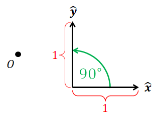
The Cartesian coordinate system specifies how to represent points and vectors in the 2D plane with two real numbers. It has three components.
- A fixed point $O$ in the plane, called the origin.
- A unit vector $\hat{\mathbf{x}}$ in the plane.
- Another unit vector $\hat{\mathbf{y}}$ in the plane such that the (signed) angle from $\hat{\mathbf{x}}$ to $\hat{\mathbf{y}}$ is $90^\circ$ ($\pi/2$ radians).
We typically draws the vector $\hat{\mathbf{x}}$ horizontally pointing to the right, and the vector $\hat{\mathbf{y}}$ vertically pointing upward.
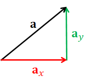
Given a vector $\mathbf{a}$ that lies in the 2D plane, we can always write $\mathbf{a}$ as a sum of two vectors $$\mathbf{a} = \mathbf{a}_x + \mathbf{a}_y$$ where $\mathbf{a}_x$ is parallel to $\hat{\mathbf{x}}$ (i.e., $\mathbf{a}_x$ is horizontal), and $\mathbf{a}_y$ is parallel to $\hat{\mathbf{y}}$ (i.e., $\mathbf{a}_y$ is vertical) as in Figure 4.2.
Because $\mathbf{a}_x$ is perpendicular to $\mathbf{a}$, we can find a real number $a_x$ such that $$\mathbf{a}_x = a_x \hat{\mathbf{x}}.$$ In particular, because $\hat{\mathbf{x}}$ is a unit vector, it should be clear that $$ \begin{align*} a_x &= \begin{cases} \| \mathbf{a}_x \|, & \mathrm{if\ }\mathbf{a}_x\mathrm{\ points\ to\ the\ right}, \\ 0, & \mathrm{if\ }\mathbf{a}_x = \mathbf{0},\\ -\| \mathbf{a}_x \|, & \mathrm{if\ }\mathbf{a}_x\mathrm{\ points\ to\ the\ left} \end{cases} \\ &= \mathrm{signed\ length\ of\ projection\ of\ \mathbf{a}\ on\ \hat{\mathbf{x}}}. \end{align*} $$ Similarly, we can say that $$\mathbf{a}_y = a_y \hat{\mathbf{y}}$$ where $$ \begin{align*} a_y &= \begin{cases} \| \mathbf{a}_y \|, & \mathrm{if\ }\mathbf{a}_y\mathrm{\ points\ upward}, \\ 0, & \mathrm{if\ }\mathbf{a}_y = \mathbf{0},\\ -\| \mathbf{a}_x \|, & \mathrm{if\ }\mathbf{a}_y\mathrm{\ points\ downward} \end{cases} \\ &= \mathrm{signed\ length\ of\ projection\ of\ \mathbf{a}\ on\ \hat{\mathbf{y}}}. \end{align*} $$ Putting this together, we have that $$ \mathbf{a} = a_x \hat{\mathbf{x}} + a_y \hat{\mathbf{y}}. $$ So, given any vector $\mathbf{a}$, we can find a pair of real numbers $(a_x, a_y)$ that satisfies the above equation. Moreover, given a pair $(a_x, a_y)$, we can use the equation to create a 2D vector. As a result, it makes sense to just represent the vector $\mathbf{a}$ with the tuple $(a_x, a_y)$. As such, we may simply write $$ \mathbf{a} = (a_x, a_y). $$ Another popular way to write the above expression is to use the column vector notation, $$ \mathbf{a} = \begin{bmatrix} a_x \\ a_y \end{bmatrix}, $$ where the numbers are arranged vertically in a square bracket. The numbers $a_x$ and $a_y$ are called the Cartesian coordinates of $\mathbf{a}$. We call $a_x$ the $x$-coordinate$ and $a_y$ the $y$-coordinate.
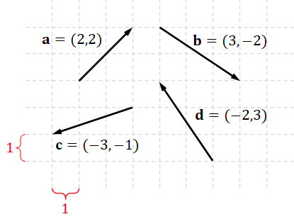
Before going further, let us take stock. What we have discussed so far is that we can represent any vector in 2D with two numbers. When we write $\mathbf{a} = (a_x, a_y)$, we mean that $\mathbf{a}$ is a vector whose (signed) horizontal length is $a_x$ and whose (signed) vertical length is $a_y$. Figure 4.3 should reinforce this intuition.
We should remember the Cartesian coordinates of well-known vectors. $$ \begin{align*} \mathbf{0} &= (0,0) = \begin{bmatrix} 0 \\ 0 \end{bmatrix}, \\ \hat{\mathbf{x}} &= (1,0) = \begin{bmatrix} 1 \\ 0 \end{bmatrix}, \\ \hat{\mathbf{y}} &= (0,1) = \begin{bmatrix} 0 \\ 1 \end{bmatrix}. \end{align*} $$
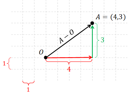
We have spoken at length how to represent vectors in the Cartesian coordinate system. Let us now turn to how to represent points, which relies heavily on the vector represention. For any point $A$ in the 2D plane, we have that $A - O$ is a 2D vector. We simply say that the Cartesian coordinates of point $A$ is simply the Cartesian coordinates of $O-A$. In other words, if $A - O = (A_x,A_y)$, then we simply say that $A = (A_x, A_y)$.
It follows that, if $A = (A_x, A_y)$, then $A_x$ is the signed distance from $O$ to $A$ in the horizontal direction. Similarly, $A_y$ is the signed distance from $O$ to $A$ in the vertical direction.
Because $O - O = \mathbf{0} = (0,0)$, it follows that the Cartesian coordinates of $O$ is $(0,0)$.
Because points and vectors in 2D can be represented by a pair of real number, we typically denote the 2D space with the symbol $\mathbb{R}^2$, which denotes the set $$ \mathbb{R}^2 = \{ (x,y) : x \in \mathbb{R}, y \in \mathbb{R} \}. $$
4.1.2 3D case
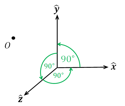
The 3D Cartesian coordinate system is very similar to the 2D system. We still have the origin $O$, which is now in a 3D space. We still have the unit vector $\hat{\mathbf{x}}$ and $\hat{\mathbf{y}}$, which are still perpendiular to one another like in the 2D case. The only addition is another unit vector $\hat{\mathbf{z}}$, which is perpendicular to both $\hat{\mathbf{x}}$ and $\hat{\mathbf{y}}$. We also require that $$\hat{\mathbf{z}} = \hat{\mathbf{x}} \times \hat{\mathbf{y}}.$$ The pieces that are used to defined a 3D Cartesian coordinate system are depicted in Figure 4.5.
Following the 2D case, any 3D vector $\mathbf{a}$ can be written as a linear combination of $\hat{\mathbf{x}}$, $\hat{\mathbf{y}}$, and $\hat{\mathbf{z}}$: $$ \mathbf{a} = a_x \hat{\mathbf{x}} + a_y \hat{\mathbf{y}} + a_z \hat{\mathbf{z}} $$ where $a_x$, $a_y$, and $a_z$ are real numbers that are equal to the signed length of the projection of $\mathbf{a}$ onto $\hat{\mathbf{x}}$, $\hat{\mathbf{y}}$, and $\hat{\mathbf{z}}$, respectively. We represent this vector with the triple $$(a_x, a_y, a_z)$$ and also denote it by the column vector notation $$\begin{bmatrix} a_x \\ a_y \\ a_z \end{bmatrix}.$$ In other words, $$ \begin{align*} (a_x, a_y, a_z) = \begin{bmatrix} a_x \\ a_y \\ a_z \end{bmatrix} = a_x \hat{\mathbf{x}} + a_y \hat{\mathbf{y}} + a_z \hat{\mathbf{z}} \end{align*} $$ We still call $a_x$ and $a_y$ the $x$-coordinate and the $y$-coordinate, respectively. Obviously, $a_z$ is called the $z$-coordinate of $\mathbf{a}$.
It follows that $$ \begin{align*} \hat{\mathbf{x}} &= (1,0,0) = \begin{bmatrix} 1 \\ 0 \\ 0 \end{bmatrix}, \\ \hat{\mathbf{y}} &= (0,1,0) = \begin{bmatrix} 0 \\ 1 \\ 0 \end{bmatrix}, \\ \hat{\mathbf{z}} &= (0,0,1) = \begin{bmatrix} 0 \\ 0 \\ 1 \end{bmatrix}. \end{align*} $$
Representation of points also follows the same system as the 2D case. We represent point $A$ in 3D space with the triple $(A_x, A_y, A_x)$ if $A - O = (A_x, A_y, A_z)$. This means that, in the 3D case, $O = (0,0,0)$.
Because points and vectors in 3D space can be represented by a triple of 3 real numbers, we refer the the 3D space with the symbol $\mathbb{R}^3$, which denotes the set $$ \mathbb{R}^3 = \{ (x,y,z) : x \in \mathbb{R}, y \in \mathbb{R}, z \in \mathbb{R} \}. $$
4.2 Vector arithmetic in the cartesian coordinate system
Using the Cartesian coordinate system, we now have a way to represent points and vectors with a collection of real numbers, which means we can store them in a computer and transmit them over a network. To do computer graphics, however, we also need ways to easily perform mathematical operations discussed in the last chapter on these representations. We shall discuss these methods in this section, focusing on the 3D vectors and points. (Operations for the 2D cases can be obtained by just dropping the $z$-coordinate.)
To faciliate the discussion that follows, let $\mathbf{a}$ and $\mathbf{b}$ be vectors in $\mathbb{R}^3$ with Cartesian coordinates $(a_x, a_y, a_z)$ and $(b_x, b_y, b_z)$, respectively. Moreover, let $c$ be an arbitrary real number.
4.2.1 Scaling
The Cartesian coordinates of the scaled vector $c\mathbf{a}$ is given by $$ \begin{align*} c\mathbf{a} = (ca_x, ca_y, ca_z) = \begin{bmatrix} ca_x \\ ca_y \\ ca_z \end{bmatrix}. \end{align*} $$ In other words, to scale a vector by a constant $c$, just multiple all of its coordinates by $c$.
4.2.2 Addition and subtraction
The Cartesian coordinates of the sum $\mathbf{a} + \mathbf{b}$ and the difference $\mathbf{a} - \mathbf{b}$ are given by: $$ \begin{align*} \mathbf{a} + \mathbf{b} &= (a_x + b_x,\ a_y + b_y,\ a_z + b_z) = \begin{bmatrix} a_x + b_x \\ a_y + b_y \\ a_z + b_z \end{bmatrix}, \\ \mathbf{a} - \mathbf{b} &= (a_x - b_x,\ a_y - b_y,\ a_z - b_z) = \begin{bmatrix} a_x - b_x \\ a_y - b_y \\ a_z - b_z \end{bmatrix}. \end{align*} $$ In other words, vector addition and subtraction are just component-wise addition and subtraction.
4.2.3 Dot product
The value of the dot product $\mathbf{a} \cdot \mathbf{b}$ is given by $$ \begin{align*} \mathbf{a} \cdot \mathbf{b} = a_x b_x + a_y b_y + a_z b_z. \end{align*} $$ In other words, multiply coordinates of the same components together and add up all the products. This means that $$ \begin{align*} \| \mathbf{a} \|^2 = \mathbf{a} \cdot \mathbf{a} = a_x^2 + a_y^2 + a_z^2. \end{align*} $$ One may recall that the above statement is just the Pythagorean theorem applied to side lengths of $a_x$, $a_y$, and $a_z$. From the above equation, we can derive the formula for the length of $\mathbf{a}$, $$ \begin{align*} \| \mathbf{a} \| = \sqrt{a_x^2 + a_y^2 + a_z^2}, \end{align*} $$ and the formula for the angle $\theta$ between $\mathbf{a}$ and $\mathbf{b}$, $$ \begin{align*} \cos\theta = \pm \arccos\bigg( \frac{\mathbf{a} \cdot \mathbf{b}}{ \| \mathbf{a} \| \| \mathbf{b} \|} \bigg) = \pm \arccos\bigg( \frac{a_x b_x + a_y b_y + a_z b_y}{\sqrt{(a_x^2 + a_y^2 + a_z^2 )(b_x^2 + b_y^2 + b_z^2)}} \bigg). \end{align*} $$
It is good to remember that the vectors $\hat{\mathbf{x}}$, $\hat{\mathbf{y}}$, and $\hat{\mathbf{z}}$, so $$\|\hat{\mathbf{x}} \| = \|\hat{\mathbf{y}} \| = \|\hat{\mathbf{z}} \| = 1.$$ Moreover, they are all perpendicular to one another, so the dot products between any two of them are all zero. $$ \hat{\mathbf{x}}\cdot \hat{\mathbf{y}} = \hat{\mathbf{y}} \cdot \hat{\mathbf{z}} = \hat{\mathbf{z}} \cdot \hat{\mathbf{x}} = 0. $$
4.2.4 Cross product
The formula for the cross product is quite complicated. Let's see it in full first. $$ \begin{align*} \mathbf{a} \times \mathbf{b} = \begin{bmatrix} a_y b_z - b_y a_z \\ a_z b_x - b_z a_x \\ a_x b_y - b_x a_y \end{bmatrix} \end{align*} $$
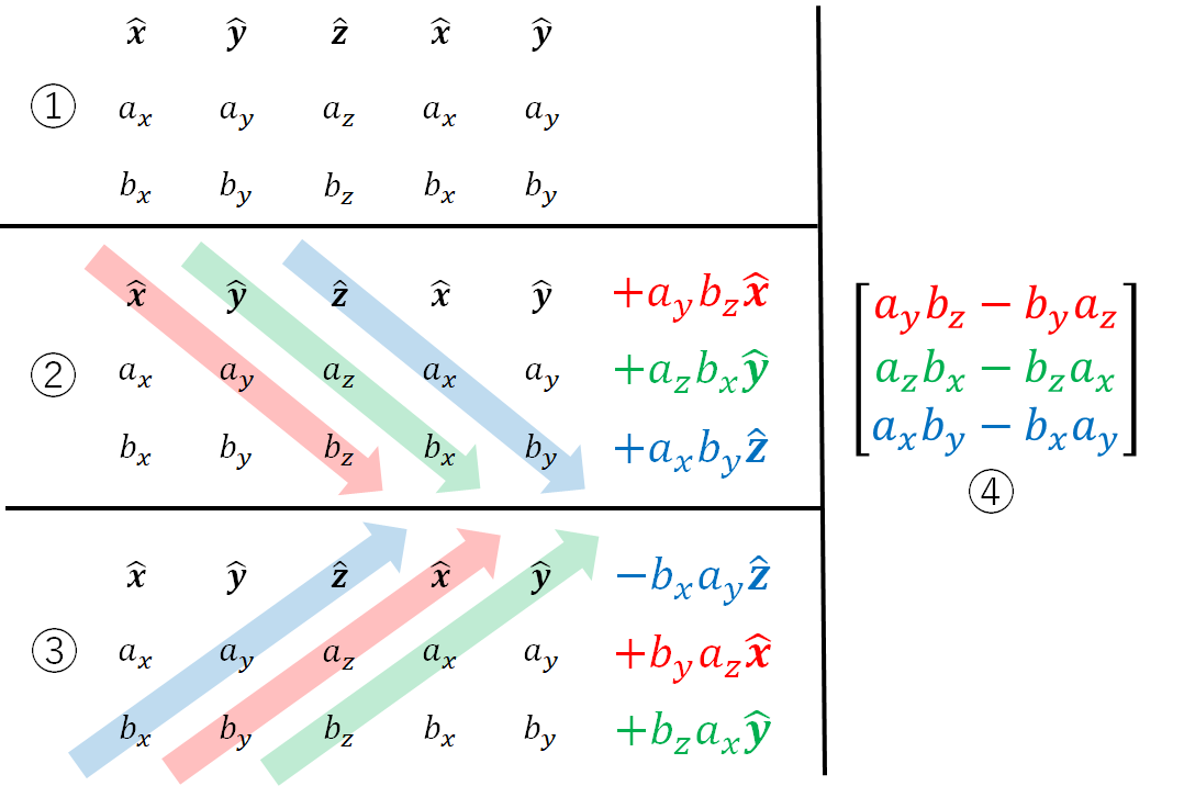
The way to remember the formula is to use the procedure outlined in Figure 4.6.
-
Write down a grid of size $3 \times 5$ like in Step ①. The first row has the unit vectors, the second row has the coordinates of $\mathbf{a}$, and the last row has the coordinates of $\mathbf{b}$. The columns goes from $x$, $y$, $z$, and then back to $x$ and $y$.
-
Draw three downward arrows like in Step ②. Multiply all the numbers/vectors under the arrows to form three terms, all of which should have positive sign.
-
Draw three upward arrows like in Step ③. Again, multiply all the numbers/vectors under the arrows to get three terms. A negative sign should be added to each of these terms.
-
Collect the expressions that are multipled to the same unit vector together.
One thing to be careful about is that the formula for cross product only works in a 3D space. If you wish to muliple two 2D vectors such as $(a_x,a_y)$ and $(b_x, b_z)$ together, you have to take them to the 3D space first. This can be done by setting the $z$-components to $0$. The calculation then goes as follows: $$ \begin{align*} \begin{bmatrix} a_x \\ a_y \\ 0 \end{bmatrix} \times \begin{bmatrix} b_x \\ b_y \\ 0 \end{bmatrix} = \begin{bmatrix} 0 \\ 0 \\ a_x b_y - b_x a_y \end{bmatrix} \end{align*} $$ The cross products between the unit vectors $\hat{\mathbf{x}}$, $\hat{\mathbf{y}}$, and $\hat{\mathbf{z}}$ are as follows: $$ \begin{align*} \hat{\mathbf{x}} \times \hat{\mathbf{y}} &= \hat{\mathbf{z}}, & \hat{\mathbf{y}} \times \hat{\mathbf{x}} &= -\hat{\mathbf{z}}, \\ \hat{\mathbf{y}} \times \hat{\mathbf{z}} &= \hat{\mathbf{x}}, & \hat{\mathbf{z}} \times \hat{\mathbf{y}} &= -\hat{\mathbf{x}}, \\ \hat{\mathbf{z}} \times \hat{\mathbf{x}} &= \hat{\mathbf{y}}, & \hat{\mathbf{x}} \times \hat{\mathbf{z}} &= -\hat{\mathbf{y}}. \end{align*} $$ A way to remember these relations is to observe that the cross product of two of the vectors are always equal to the vector that is left out. If the two vectors follows the sequence $\hat{\mathbf{x}} \rightarrow \hat{\mathbf{y}} \rightarrow \hat{\mathbf{z}} \rightarrow \hat{\mathbf{x}}$, then the result is positive. On the other hand, if the order in the opposite direction ($\hat{\mathbf{x}} \rightarrow \hat{\mathbf{z}} \rightarrow \hat{\mathbf{y}} \rightarrow \hat{\mathbf{x}}$), then the result is negative.
4.2.5 Point arithmetic
We perform arithmetic operations on points in the exact same way as we perfrom those operations on vectors. Nevertheless, one needs to keep track of what the three numbers are representing and only applies valid operations to them. As we discussed in the last chapter, only three operations are allowed on points:
- point-vector addition,
- point-point subtraction, and
- linear combinations of points where the coefficients add up to $1$.
As a result, it makes sense to compute $$ \begin{align*} \begin{bmatrix} 1 \\ 2 \\ 3 \end{bmatrix}_{\mathrm{point}} + \begin{bmatrix} 4 \\ 5 \\ 6 \end{bmatrix}_{\mathrm{vector}} &= \begin{bmatrix} 5 \\ 7 \\ 9 \end{bmatrix}_{\mathrm{point}}, \\ \begin{bmatrix} 1 \\ 5 \\ 2 \end{bmatrix}_{\mathrm{point}} - \begin{bmatrix} 3 \\ 1 \\ 0 \end{bmatrix}_{\mathrm{point}} &= \begin{bmatrix} -2 \\ 4 \\ 2 \end{bmatrix}_{\mathrm{vector}}, \\ 0.2 \begin{bmatrix} 0 \\ 1 \\ 0 \end{bmatrix}_{\mathrm{point}} + 0.8 \begin{bmatrix} 1 \\ 0 \\ 1 \end{bmatrix}_{\mathrm{point}} &= \begin{bmatrix} 0.8 \\ 0.2 \\ 0.8 \end{bmatrix}_{\mathrm{point}}, \end{align*} $$ but it does not make sense to compute $$ \begin{align*} \begin{bmatrix} 1 \\ 2 \\ 3 \end{bmatrix}_{\mathrm{point}} + \begin{bmatrix} 4 \\ 5 \\ 6 \end{bmatrix}_{\mathrm{point}} & & (\mathrm{the}\ \mathrm{coefficients}\ \mathrm{adds}\ \mathrm{to}\ 2\ \mathrm{instead}\ \mathrm{of}\ 1), \\ \begin{bmatrix} 1 \\ 2 \\ 3 \end{bmatrix}_{\mathrm{point}} \times \begin{bmatrix} 4 \\ 5 \\ 6 \end{bmatrix}_{\mathrm{point}} & & (\mathrm{the}\ \mathrm{cross}\ \mathrm{product}\ \mathrm{between}\ \mathrm{points}\ \mathrm{is}\ \mathrm{not}\ \mathrm{defined }). \end{align*} $$
4.3 Homogeneous coordinates
We just learned that representing points and vectors by their Cartesian coordinates allows us to perform calcalution on them with a computer. Nevertheless, the system is not very convenient because we need to keep track of whether the three numbers we operate on represent a point or a vector. It would be really nice if we have a way to distinguish between points and vectors in the data itself.
Homogeneous coordinates allows us to do just that. Given Cartesian coordinates $(x,y,z)$, the corresponding homogeneous coordinate is $$ (x,y,z,0) $$ if it represents a vector and $$ (x,y,z,1) $$ if it represents a point. In other words, we use a tuple of 4 real numbers to represent a point or a vector. The first three numbers are the $x$-, $y$-, and $z$-coordinates, and the last number tells us the data type.
Just like Cartesian coordinates, we perform scaling, addition, and subtraction on homogeneous coordinates by performing the operations on the components independently of one another. The fourth number of the result will tell us whether the operation is valid or not.
- If the resulting fourth number is $0$, the data represent a vector.
- If the resulting fourth number is $1$, the data represent a point.
- If the resulting fourth number is anything else, the operation was not valid and should not be performed in the first place.
As a result, one can always add or subtract two vectors together because the resulting fourth number will always be zero. $$ \begin{align*} \begin{bmatrix} a_x \\ a_y \\ a_z \\ 0 \end{bmatrix} + \begin{bmatrix} b_x \\ b_y \\ b_z \\ 0 \end{bmatrix} &= \begin{bmatrix} a_x + b_x \\ a_y + b_y \\ a_z + b_z \\ 0 \end{bmatrix}, & \begin{bmatrix} a_x \\ a_y \\ a_z \\ 0 \end{bmatrix} - \begin{bmatrix} b_x \\ b_y \\ b_z \\ 0 \end{bmatrix} &= \begin{bmatrix} a_x - b_x \\ a_y - b_y \\ a_z - b_z \\ 0 \end{bmatrix}. \end{align*} $$ It is also OK to add a point to a vector and to subtract a point from antoher point. $$ \begin{align*} \begin{bmatrix} a_x \\ a_y \\ a_z \\ 1 \end{bmatrix} + \begin{bmatrix} b_x \\ b_y \\ b_z \\ 0 \end{bmatrix} &= \begin{bmatrix} a_x + b_x \\ a_y + b_y \\ a_z + b_z \\ 1 \end{bmatrix}, & \begin{bmatrix} a_x \\ a_y \\ a_z \\ 1 \end{bmatrix} - \begin{bmatrix} b_x \\ b_y \\ b_z \\ 1 \end{bmatrix} &= \begin{bmatrix} a_x - b_x \\ a_y - b_y \\ a_z - b_z \\ 0 \end{bmatrix}. \end{align*} $$ Nevertheless, it is not OK to directly add two points togther because the fourth number will be $2$ insteadof $1$. $$ \begin{bmatrix} a_x \\ a_y \\ a_z \\ 1 \end{bmatrix} + \begin{bmatrix} b_x \\ b_y \\ b_z \\ 1 \end{bmatrix} = \begin{bmatrix} a_x + b_x \\ a_y + b_y \\ a_z + b_z \\ 2 \end{bmatrix} \qquad (\mathrm{invalid}\ \mathrm{operation}). $$ However, if the coefficients before the points add up to $1$, then the fourth number will be $1$, which means the result is a valid point. $$ (1-\alpha) \begin{bmatrix} a_x \\ a_y \\ a_z \\ 1 \end{bmatrix} + \alpha \begin{bmatrix} b_x \\ b_y \\ b_z \\ 1 \end{bmatrix} = \begin{bmatrix} (1- \alpha)a_x + \alpha b_x \\ (1 - \alpha)a_y + \alpha b_y \\ (1- \alpha) a_z + \alpha b_z \\ (1 - \alpha) + \alpha \end{bmatrix} = \begin{bmatrix} (1- \alpha)a_x + \alpha b_x \\ (1 - \alpha)a_y + \alpha b_y \\ (1- \alpha) a_z + \alpha b_z \\ 1 \end{bmatrix}. $$ Lastly, one can multiply a vector to any real number. $$ \begin{align*} c \begin{bmatrix} a_x \\ a_y \\ a_z \\ 0 \end{bmatrix} = \begin{bmatrix} c a_x \\ c a_y \\ c a_z \\ 0 \end{bmatrix} \end{align*} $$ However, scaling a point is generally not allowed unless scaling factor is $0$ or $1$. $$ \begin{align*} c \begin{bmatrix} a_x \\ a_y \\ a_z \\ 1 \end{bmatrix} = \begin{bmatrix} c a_x \\ c a_y \\ c a_z \\ c \end{bmatrix} \qquad (\mathrm{invalid}\ \mathrm{operation}\ \mathrm{if}\ c \neq 0\ \mathrm{and}\ c \neq 1) \end{align*} $$ For this book, we shall not define dot products and cross products directly on homogeous coordinates. So, when asked to perform these operations on them, we need to check whether the fourth numbers of the operands are zeros. If so, we can perform the operations on the first three numbers to get the result. For the dot product, the result is a real number, and we do not have to do anything further. $$ \begin{align*} \begin{bmatrix} a_x \\ a_y \\ a_z \\ 0 \end{bmatrix} \cdot \begin{bmatrix} b_x \\ b_y \\ b_z \\ 0 \end{bmatrix} = a_x b_x + a_y b_y + a_z c_z. \end{align*} $$ For the cross product, we will get three numbers as a result, and we have to add $0$ as the fourth number to make the result a homogeneous coordinate again. $$ \begin{align*} \begin{bmatrix} a_x \\ a_y \\ a_z \\ 0 \end{bmatrix} \times \begin{bmatrix} b_x \\ b_y \\ b_z \\ 0 \end{bmatrix} = \begin{bmatrix} a_y b_z - b_y a_z \\ a_z b_x - b_z a_x \\ a_x b_y - a_y b_x \\ 0 \end{bmatrix}. \end{align*} $$
4.3.1 Interpretation of homogeneous coordinates
In general, the homogeneous coordinates $(a_x, a_y, a_z, a_w)$ can be understood as follows: $$ \begin{align*} \begin{bmatrix} a_x \\ a_y \\ a_z \\ a_w \end{bmatrix} \qquad \mathrm{corresponds}\ \mathrm{to} \qquad a_x \hat{\mathbf{x}} + a_y \hat{\mathbf{y}} + a_z \hat{\mathbf{z}} + a_w O. \end{align*} $$
We see that $a_x \hat{\mathbf{x}} + a_y \hat{\mathbf{y}} + a_z \hat{\mathbf{z}}$ is always a vector. The expression $a_w O$ is valid only if $a_w = 1$, in which $a_w O = O$. However, we will make a new exception and set $a_w O$ to be the zero vector if $a_w = 0$. Note that this is consistent with the fact that $0(a_x, a_y, a_z, a_w) = (0,0,0,0)$, which is the zero vector no matter what $a_w$ is.
This interpretation puts emphasis on the numbers in homogeneous coordinates as scaling factors of geometric entities.
- $a_x$ is the scaling factor of the vector $\hat{\mathbf{x}}$.
- $a_y$ is the scaling factor of the vector $\hat{\mathbf{y}}$.
- $a_z$ is the scaling factor of the vector $\hat{\mathbf{z}}$.
- $a_w$ is the scaling factor of the point $O$.
(However, unlike the vectors, the point $O$ can only be scaled by $0$ or $1$.) After being scaled, these entities are added together to form an expression, which evaluates to either a point or a vector.
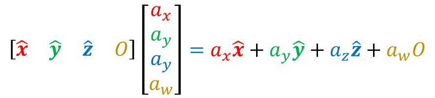
Another way to interpret the homogeneous coordinate is to think that it is always implicitly multiplied by the matrix $\begin{bmatrix} \hat{\mathbf{x}} & \hat{\mathbf{y}} & \hat{\mathbf{z}} & O \end{bmatrix}$. In other words, $$ \begin{align*} \begin{bmatrix} a_x \\ a_y \\ a_z \\ a_w \end{bmatrix} \qquad \mathrm{corresponds}\ \mathrm{to} \qquad \begin{bmatrix} \hat{\mathbf{x}} & \hat{\mathbf{y}} & \hat{\mathbf{z}} & O \end{bmatrix} \begin{bmatrix} a_x \\ a_y \\ a_z \\ a_w \end{bmatrix} \end{align*} $$ The expression on the right is a product of two matrices. We will discuss matrix multiplication in more details in Chapter 13. For now, it suffices to do the computation according to Figure 4.7, and the result would be exactly $a_x \hat{\mathbf{x}} + a_y \hat{\mathbf{y}} + a_z \hat{\mathbf{z}} + a_w O$.
4.3.2 Homogeneous coordinates for 2D points and vectors
The homogeneous coordinates for points and vectors in $\mathbb{R}^2$ is similar to those in $\mathbb{R}^3$. Given Cartesian coordinates $(x,y)$, its homogeneous coordinate is $(x,y,1)$ if it represents a point and $(x,y,0)$ if it represents a vector. In general, we have that $$ \begin{align*} \begin{bmatrix} a_x \\ a_y \\ a_w \end{bmatrix} \qquad \mathrm{corresponds}\ \mathrm{to} \qquad \begin{bmatrix} \hat{\mathbf{x}} & \hat{\mathbf{y}} & O \end{bmatrix} \begin{bmatrix} a_x \\ a_y \\ a_w \end{bmatrix} = a_x \hat{\mathbf{x}} + a_y \hat{\mathbf{y}} + a_w O. \end{align*} $$
The number can be intepreted in the same way as in the 3D case.
- $a_x$ is the scaling factor of the vector $\hat{\mathbf{x}}$.
- $a_y$ is the scaling factor of the vector $\hat{\mathbf{y}}$.
- $a_w$ is the scaling factor of the point $O$.
The rules for manipulating 2D homogeneous coordinates are the same as 3D ones: scaling and adding the components independently. Moreover, as usual, the dot product and the cross products needs to be dealt with in special ways. Most importantly, computing cross products of two 2D vectors results in a 3D vector, and the result cannot be represented with homogeneous coordinates for a 2D vector. Hence, we suggest the reader to lift 2D vectors into 3D spaces (by setting the $z$-coordinate to $0$) before computing any cross products.
4.4 Affine coordinate system
The affine coordinate system is a generalization of the Cartesian coordinate system. It is used very frequently in computer graphics. While computer graphics usually use 3D affine coordinate system, it is much easier to introduce the concept with the 2D version. So, we will mainly discuss the 2D version in this section.
Let us recapitulate what we discussed in the last section. The 2D Cartesian coordinate system is defined with an origin point $O$ and two perpedicular unit vectors $\hat{\mathbf{x}}$ and $\hat{\mathbf{y}}$. With homogeneous coordinates, points and vectors are represented by a tuple of 3 numbers according to the following rules. $$ \begin{align*} \begin{bmatrix} a_x \\ a_y \\ a_w \end{bmatrix} \qquad \mathrm{represents} \qquad \begin{bmatrix} \hat{\mathbf{x}} & \hat{\mathbf{y}} & O \end{bmatrix} \begin{bmatrix} a_x \\ a_y \\ a_w \end{bmatrix} = a_x \hat{\mathbf{x}} + a_y \hat{\mathbf{y}} + a_w O \end{align*} $$ where $a_w$ can be either $0$ (representing a vector) or $1$ (representing a point).
The 2D affine coordinate system relaxes constraints on the vectors $\hat{\mathbf{x}}$ and $\hat{\mathbf{y}}$, which are called the **basis vectors** of the coordinate system. The Cartesian coordinate system requires that they must be unit vectors, and the angle from $\hat{\mathbf{x}}$ to $\hat{\mathbf{y}}$ is $90^\circ$. The affine coordinate system do not require that they both have length 1 and that the angle is $90^\circ$. Let us say that the basis vectors are $\mathbf{x}'$ and $\mathbf{y}'$. The only requirements on them are as follows.
- Both vectors must have length greater than $0$. That is, $| \mathbf{x}' |, | \mathbf{y}' | > 0.$
- The two vectors must not be parallel. That is, you cannot find a real number $c$ such that $c\mathbf{x}' = \mathbf{y}$.
The affine coordinate system has an origin too. Because it can be different from the Cartesian coordinate systems's origin $O$, let us call it $O'$.
The rule for representing points and vectors with numbers are similar to that of the Cartesian coordinate system. We represent a point and a vector by a 3-tuple $(a_x, a_y, a_w)$ where $$ \begin{align*} \begin{bmatrix} a_x \\ a_y \\ a_w \end{bmatrix} \qquad \mathrm{represents} \qquad \begin{bmatrix} \mathbf{x}' & \mathbf{y}' & O' \end{bmatrix} \begin{bmatrix} a_x \\ a_y \\ a_w \end{bmatrix} = a_x \mathbf{x}' + a_y \mathbf{y}' + a_w O' \end{align*} $$ with $a_w$ can either be $0$ or $1$. In other words, we just replace $O$ with $O'$, $\hat{\mathbf{x}}$ with $\mathbf{x}'$, and $\hat{\mathbf{y}}$ with $\mathbf{y}'$.
Because the basis vectors and the origin of an affine coordinate system are in general different from those of the Cartesian coordinate system, the same tuple of numbers $(a_x, a_y, a_w)$ can represent different points and vectors depending on the coordinate system used to interpret them. We can visualize this fact by drawing the lattice grid of the coordinate systems. That is:
- we draws lines for points of the form $(x,0,1)$, $(x, \pm 1, 1)$, $(x, \pm 2, 1)$, $(x, \pm 3, 1)$ and so on where the $x$-coordinate is allowed to vary freely, and the $y$-coordinate is only allowed to be integers, and
- we draw lines for points of the form $(0,y,1)$, $(\pm 1,y,1)$, $(\pm 2,y,1)$, $(\pm 3,y,1)$ and so on where the $x$-coordinate is allowed to vary freely, and the $y$-coordinate is only allowed to be integers.
The points where the lines cross are called lattice points. These are points whose coordinates are integers. The lattice grid illustrate the "shape" of the coordinate systems.
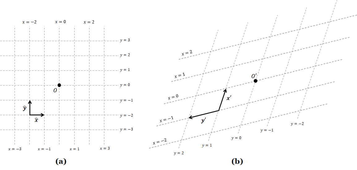
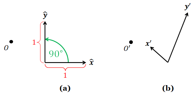
We can see in Figure 4.9 that they are different. For the Cartesian coordinate system (4.9a), the 2D plane is divided into grid cells, each of which is a square. However, for the affine coordinate system in Figure 4.9b, the grid cells are parallelograms. Notice also that, because the basis vectors are allowed to point in any directions, the directions in which the $x$-coordinate and $y$-coordinate increase can be arbitrary. In Figure 4.9b, the $x$-coordinate increases as we go up, and the $y$-coordinte increases as we go left. This behavior is very different from the Cartesian coordinate system.
Looking at Figure 4.9, we can see the importance of the constraints placed on $\mathbf{x}'$ and $\mathbf{y}'$. If one of the vectors have length $0$, then the grid lines for the corresponding coordinate would collapse to a single line, and the points that can be represented by the coordinates system would consist of those on the line corresponding to non-zero vector, not the whole plane. (Mathematically, we say that the $\mathbf{x}'$ and $\mathbf{y}'$ does not span the whole 2D plane.) The same thing happens if the two vectors are parallel to each other.
It should also become clear that there are many affine coordinate systems because we have much more freedom in the way we chooose $\mathbf{x}'$ and $\mathbf{y}'$. On the other hand, we tend to think that there is only one Cartesian coordinate system for each fixed number of dimensions. This is not quite true because we can move the origin $O$ around and rotate $\hat{\mathbf{x}}$ arbitrarily. However, once we fix $O$ and $\hat{\mathbf{x}}$, it becomes the reference points from which we can describe other affine coordinate system. We will discuss conversion between coordinate systems in Chapter 13.
4.4.1 3D affine coordinate systems
For a 3D affine coordinate system, we need another a third basis vector $\mathbf{z}'$. The constraints on the basis vectors are:
- All vectors must have length greater than $0$: $\|\mathbf{x}'\|, \|\mathbf{y}'\|, \| \mathbf{z}' \| > 0$.
- All vectors must not lie in the same plane.
The two conditions are to ensure that the basis vectors span the whole 3D space. Again, points and vectors can be represented by affine coordinates $(a_x, a_y, a_z, a_w)$ according to the following rule: $$ \begin{align*} \begin{bmatrix} a_x \\ a_y \\ a_z \\ a_w \end{bmatrix} \qquad \mathrm{represents} \qquad \begin{bmatrix} \mathbf{x}' & \mathbf{y}' & \mathbf{z}' & O' \end{bmatrix} \begin{bmatrix} a_x \\ a_y \\ a_w \end{bmatrix} = a_x \mathbf{x}' + a_y \mathbf{y}' + a_z \mathbf{z}' + a_w O'. \end{align*} $$
4.4.2 Vector and point arithmetic in affine coordinate systems
We saw in the last section that, all arithmetic operations (addition, scalar multiplication, dot prodcut, cross product) on Cartesian coordinates are meaningful, and they correspond to arithmetic operations on points and vectors discussed in the last section. This fact, however, is not the case in other coordinate systems where some calculations on the coordinates are meaningful, and some are not (in other words, they lead to inccorect results).
For the affine coordinate system, addition, subtraction, and scalar multiplication are meaningful, but operations that involve length such as dot product and cross product are not. Let us discuss the operations one by one.
Addition and scalar multiplication. Let $(a_x, a_y, a_z, a_w)$ and $(b_x, b_y, b_z, b_w)$ be homogeneous coordinates in an affine coordinate system defined by the origin point $O'$ and the three axes $\mathbf{x}'$, $\mathbf{y}'$, $\mathbf{z}'$ Then, we know that \begin{align*} \begin{bmatrix} a_x \\ a_y \\ a_z \\ a_w \end{bmatrix} &\quad \mathrm{represents} \quad a_x \mathbf{x}' + a_y \mathbf{y}' + a_z \mathbf{z}' + a_w O', \quad \mathrm{and}\\ \begin{bmatrix} b_x \\ b_y \\ b_z \\ b_w \end{bmatrix} &\quad \mathrm{represents} \quad b_x \mathbf{x}' + b_y \mathbf{y}' + b_z \mathbf{z}' + b_w O'. \end{align*} Consider the linear combination \begin{align*} \alpha \begin{bmatrix} a_x \\ a_y \\ a_z \\ a_w \end{bmatrix} + \beta \begin{bmatrix} b_x \\ b_y \\ b_z \\ b_w \end{bmatrix} = \begin{bmatrix} \alpha a_x + \beta b_x \\ \alpha a_y + \beta b_y \\ \alpha a_z + \beta b_z \\ \alpha a_w + \beta b_w \end{bmatrix} \end{align*}. where $\alpha$ and $\beta$ are scalars that make the resulting homogeneous coordinates well defined (i.e, $\alpha a_w + \beta b_w$ is either $0$ or $1$.) We know that $$ \begin{align*} \begin{bmatrix} \alpha a_x + \beta b_x \\ \alpha a_y + \beta b_y \\ \alpha a_z + \beta b_z \\ \alpha a_w + \beta b_w, \end{bmatrix} &\quad \mathrm{represents} \quad (a_x + b_x) \mathbf{x}' + (a_y + b_y) \mathbf{y}' + (a_z + b_z) \mathbf{z}' + (a_w + b_w) O', \end{align*} $$ and $$ \begin{align*} &(\alpha a_x + \beta b_x) \mathbf{x}' + (\alpha a_y + \beta b_y) \mathbf{y}' + (\alpha a_z + \beta b_z) \mathbf{z}' + (\alpha a_w + \beta b_w) O' \\ &\quad = \alpha \big( a_x \mathbf{x}' + a_y \mathbf{y}' + a_z \mathbf{z}' + a_w O' \big) + \beta \big( b_x \mathbf{x}' + b_y \mathbf{y}' + b_z \mathbf{z}' + b_w O' \big). \end{align*} $$ This means that $$ \begin{align*} \alpha \begin{bmatrix} a_x \\ a_y \\ a_z \\ a_w \end{bmatrix} + \beta \begin{bmatrix} b_x \\ b_y \\ b_z \\ b_w \end{bmatrix} &\quad \mathrm{represents} \quad \alpha \big( a_x \mathbf{x}' + a_y \mathbf{y}' + a_z \mathbf{z}' + a_w O' \big) + \beta \big( b_x \mathbf{x}' + b_y \mathbf{y}' + b_z \mathbf{z}' + b_w O' \big). \end{align*} $$ We have just shown that the linear combination of homogeneous coordinates in an affine coordinate system represents the linear combination of points/vectors represented by the homogeneous coordinates that were operated upon. So, addition, subtraction, and scalar multiplication in an affine coordinate system is meaningful. We can perform these calculations on the coordinates, and they will yield sensible results.
Dot product. Computing dot products in the affine coordinate system using the formula we use for the Cartesian coordinate system does not yield correct results. For example, consider an affine coordinate system in 2D where $\| \mathbf{x}' \| = 3$ and $\| \mathbf{y}' \| = 4$ in the figure below.
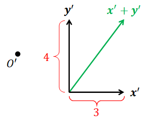
Working in non-homogenous coordinates, we know that
- $(1,0)$ represents the vector $\mathbf{x}'$.
- $(0,1)$ represents the vector $\mathbf{y}'$.
- $(1,1)$ represents the vector $\mathbf{x}' + \mathbf{y}'$.
However,
- $(1,0) \cdot (1,0) = 1 \cdot 1 = 1$, but $\mathbf{x}' \cdot \mathbf{x}' = \| \mathbf{x}' \|^2 = 3^2 = 9$.
- $(0,1) \cdot (0,1) = 1 \cdot 1 = 1$, but $\mathbf{y}' \cdot \mathbf{y}' = \| \mathbf{y}' \|^2 = 4^2 = 16$.
- $(1,1) \cdot (1,1) = 1 \cdot 1 + 1\cdot 1 = 2$, but $(\mathbf{x}' + \mathbf{y}') \cdot (\mathbf{x}' + \mathbf{y}') = \| \mathbf{x}' + \mathbf{y}' \|^2 = 3^2 + 4^2 = 25.$
We see clearly that the dot product formula $$ (a_x, a_y) \cdot (b_x, b_y) = a_x b_x + a_y b_y $$ does not work in this affine coordinate system. In fact, the formula only works in coordinate systems where *the axes vectors are of unit length and are mutually perpedicular to one another.* Such coordinate systems are called orthonormal. The Cartesian coordinate system is orthonomal, but the coordinate system in Figure 4.10 is not. In general, we must be careful not to use the dot product formula in an arbitrary affine coordinate system. The safest way is to convert affine coordinates into Cartesian coordinates first before computing a dot product. Again. we will discuss transformation between coordinate systems in Chapter 13.
Cross product. Continuing from the last example. Let us expand the coordinate system in Figure 4.10 into a 3D coordinate system by adding a vector $\mathbf{z}'$ that is perpendicular to both $\mathbf{x}'$ and $\mathbf{y}'$ with $\| \mathbf{z}' \| = 2$.
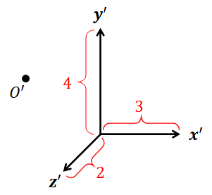
Now,
- $(1,0,0)$ represents the vector $\mathbf{x}'$.
- $(0,1,0)$ represents the vector $\mathbf{y}'$.
- $(0,0,1)$ represents the vector $\mathbf{z}'$.
The cross product formula tells us that $(1,0,0) \times (0,1,0) = (0,0,1)$. In other words, it tells us that $\mathbf{x}' \times \mathbf{y}'$ should be equal to $\mathbf{z}'$. This implies that $$\|\mathbf{x}' \times \mathbf{y}' \| \stackrel{?}{=} \| \mathbf{z}' \| \stackrel{?}{=} 2.$$ However, the assertion is far from the truth because $$ \begin{align*} \| \mathbf{x}' \times \mathbf{y}' \| = \| \mathbf{x}' \| \| \mathbf{y}' \| \sin 90^\circ = 3 \cdot 4 = 12. \end{align*} $$ This example illustrates that computing cross products in affine coordinate systems does not work correctly in general. The safest way, again, would be to convert affine coordinates into Cartesian coordinates first.
4.5 Other coordainate systems
We have discussed two coordinate systems that are frequently used in computer graphics. However, there are other coordinate systems that are widely used in other domains (mathematics, physics, engineering, etc.). We mention some of this section without studying them in details. This is to drive home the points that coordinate systems are ways to turn points and vectors into numbers, and there are many ways to do so.
4.5.1 Polar coordinate system
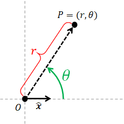
The polar coordinate system works with the 2D Euclidean space. We say that a point $P$ has polar coordinates $(r,\theta)$ if its Cartesian coordinates are $(r\cos\theta, r\sin\theta)$. In other words, $$ \begin{align*} \begin{bmatrix} r \\ \theta \end{bmatrix}_{\mathrm{polar}} = \begin{bmatrix} r\cos\theta \\ r\sin\theta \end{bmatrix}_{\mathrm{Cartesian}}. \end{align*} $$ The number $r$ is the distance between $P$ and the origin $O$, and the number $\theta$ is the angle from the basis vector $\hat{\mathbf{x}}$ to the vector $P - O$.
4.5.2 Cylindrical coordinate system
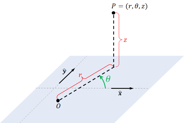
The cylindrical coordinate system is a straightforward extension of the polar coordinate system in order to represent points in the 3D Euclidean space. We say that a 3D point $P$ has cylindrical coordinates $(r, \theta, z)$ if its 3D Cartesian coordinates are $(r\cos\theta, r\sin\theta, z)$. Symbolically, $$ \begin{align*} \begin{bmatrix} r \\ \theta \\ z \end{bmatrix}_{\mathrm{cylindrical}} = \begin{bmatrix} r\cos\theta \\ r\sin\theta \\ z \end{bmatrix}_{\mathrm{Cartesian}}. \end{align*} $$ In other words, the cylindrical coordinate system adds a third number of polar coordinates to represent position along the third dimension.
4.5.3 Spherical coordinate system
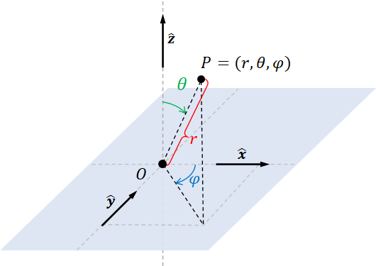
The spherical coordinate system gives another way to represent points in the 3D Euclidean space. We say that poinat $P$ has spherical coordinates $(r,\theta,\varphi)$ if its 3D Cartesian coordinates are given by $(r\sin\theta\cos\varphi, r\sin\theta\sin\varphi, r\cos\theta)$. In other words, $$ \begin{align*} \begin{bmatrix} r \\ \theta \\ \varphi \end{bmatrix}_{\mathrm{spherical}} = \begin{bmatrix} r\sin\theta\cos\varphi \\ r\sin\theta\cos\varphi \\ r\cos\theta \end{bmatrix}_{\mathrm{Cartesian}}. \end{align*} $$ Here, $r$ is the distance between $P$ and the origin $O$. The angle $\theta$ is called the polar angle, and it is the angle from the $\hat{\mathbf{z}}$ vector to the vector $P - O$. The angle $\varphi$ is called the azimuthal angle, and it is the angle from the $\hat{\mathbf{x}}$ vector to the projection of $P - O$ onto the $xy$-plane.
4.6 Summary
- A coordinate system is a way to represent a point (or a vector) with a finite sequence of numbers. Such numbers are called the point's (or the vector's) coordinates. We need a coordinate system in order to be able to do calculations on these geometric concepts with a computer.
- The Cartesian coordinate system is considered the standard coordinate system that can be used to represent points and vectors in the Euclidean space. It is defined by an origin point $O$ and a collection of basis vectors that are perpendicular to one another. The number of basis vectors is equal to the number of dimensions of the Euclidean space: 2 ($\hat{\mathbf{x}}$ and $\hat{\mathbf{y}}$) for the 2D space, and 3 ($\hat{\mathbf{x}}$, $\hat{\mathbf{y}}$, and $\hat{\mathbf{z}}$) for the 3D space.
- Once points and vectors are represented by Cartesian coordinates, we can perform all arithmetic operations discussed in the last chapters (addition, scalar multiplication, dot product, and cross product) on the coordinates instead of relying on geometric drawing and reasoning like we did previously.
- By adding one extra number (which is either 0 or 1) to Cartesian coordinates, we get the homogeneous coordinates, which can be used to represent both points and vectors without us having to remember the type of objects were are working on. By checking the value the extra number at the end of a calculation whether it is still $0$ or $1$, we can tell whether the calculation corresponds to a valid operation on points and vectors or not.
- An affine coordinate system is a generalization of the Cartesian coordinate system in which the basis vectors are required neither to have unit lengths nor to be perpendicular to one another. Addition, subtraction, and scalar multiplication of affine coordinates always yield correct representations of resulting points. Howver, operations that involve lengths such as the dot product and the cross product will generally yield wrong answers.
- The Cartesian and affine coordinate systems are the most used coordinate systems in computer graphics. However, there are well-known other coordinate systems including the polar coordinate system, the cylindrical coordinate system, and the spherical coordinate system.