3 Space, points, and vectors
In the last chapter, we studied images, which are most of the time the final output of CG programs. In this chapter, we turn to the input. Recall that 3DCG produces images by taking photographs of virtual scenes by a virtual camera. The knowledge in this and several more chapters to come will allow us to specify both of them.
Specifying a virual scene requires us to specify shapes and where they are located. So, we need knowledge about geometry, which is precisely the branch of mathematics that deals with concepts such as shapes, positions, distances, and sizes. There are multiple ways to study geometry. In Euclidean geometry, we study concepts such as points, lines, angles, triangles, and circles through drawing figures, assigning to some of their parts, and reasoning about their properties. In analytic geometry, we assign to each point a tuple of numbers called coordinates and do computation on the coordinates directly. In linear algebra, we work with abstract notions such as vectors, matrices, and linear transformations and use them to make sense of other geometrical knowledge.
In this chapter, we will study geometry through the lens of Euclidean geometry and linear algebra. We will defer numerical representations of points and vectors until Chapter 4? where we will discuss coordinates systems in great details. The reason for doing this is to let ourselves see that geometrical concepts such as points, vectors, angles, etc. are independent of coordinate systems. In this way, I think it will become less confusing when we learn how to change one coordinate system to another.
3.1 Basic geometrical concepts
The starting point for our discussion is the Euclidean space, which should represent the 3D space that all of us inhabit. We shall refer to the Euclidean plane when we talk about geometry in two dimensions. We assume that that distance in these spaces is measured with a unit which we shall not name. It can be the meter, the centimeter, the foot, the shaku, the Planck length, or anything.
The spaces can be though of as a set of points, and a point is something that has a position but has no width, height, or depth. When thought of as sets of points, the Euclidean space is denoted by $\mathbb{R}^3$ and the Euclidean plane by $\mathbb{R}^2$.
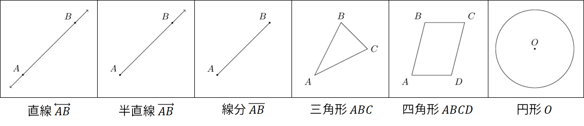
We shall be concerned with objects such as straight lines (that extends to indefinitely in both directions), rays (that starts at a point and extends indefinitely in one direction), segments (that starts from a point and ends at another), triangles, quadrileterals, and circles. We will not define these terms and assume that the reader is already familiar with them.
3.2 Angles
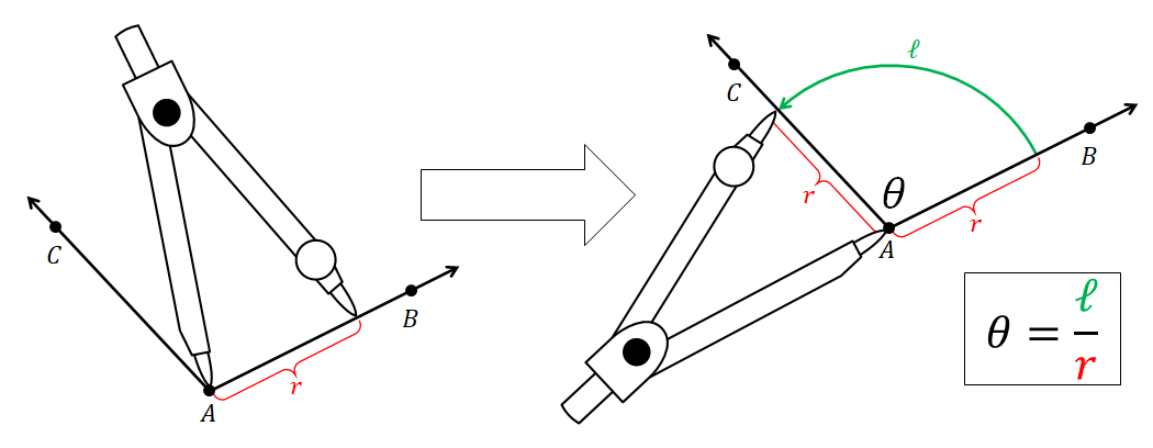
An important concept that we shall define a litte more carefully is the angle. Consider three points $A$, $B$, and $C$ such that $A \neq B$ and $A \neq C$. With them, we can form two rays $\overrightarrow{AB}$ and $\overrightarrow{AC}$. Take a compass and arrange it so that the needle point and the pencil tip are separated by some $r > 0$ unit of length. Put the needle point on $A$ and the pencil tip on the ray $\overrightarrow{AB}$. Draw a circular arc by moving the pencil tip from $\overrightarrow{AB}$ to $\overrightarrow{AC}$ while keeping the needle point at $A$. Let $\ell$ be the (non-negative) length of the drawn circular arc. Let $\theta$ be the ratio between the arc length $\ell$ and the radius $r$: $$\theta = \frac{\ell}{r}.$$ The (signed) angle from $\overrightarrow{AB}$ to $\overrightarrow{AC}$, measured in radians, is defined as follows.
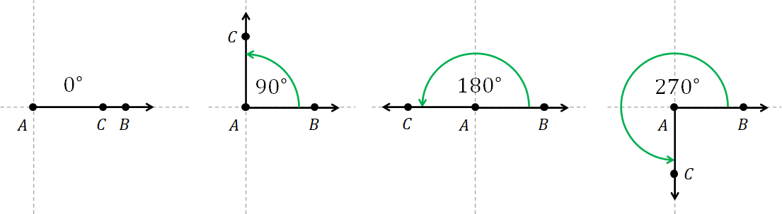
- If the motion of the compass was counterclockwise, the angle is $\theta$ radians.
- If the motion of the compass was clockwise, the angle is $-\theta$ radians.
Symbolically, we write $$ \angle(\overrightarrow{AB}, \overrightarrow{AC}) = \theta.$$
If we do not care about the direction that the compass moved, we may say that the angle between $\overrightarrow{AB}$ to $\overrightarrow{AC}$ is $\theta$ radians. Here, $\theta$ is always non-negative.
3.2.1 Units of angles
Because $\theta$ is a ratio between length and length, the unit of an angle should be nothing because the length units cancel out. As a result, the word "radians" effectively stands for "no unit" and so it is called a dimensionless unit. However, it is not OK to drop the word altogether because there's another popular unit for angles: the degree. The relationship between them is: $$ \mathrm{degree} = 180 \times \frac{\mathrm{radian}}{\pi}. $$ The angle of $d$ degrees is often denoted by $d^\circ$.
3.2.2 Equivalence between angles
The definition we have discussed so far implies that we start from $\overrightarrow{AB}$ and stop turning the compass as soon as we reach $\overrightarrow{AC}$. As a result, the arc length would the shortest. So, any angle would be in the range $(-2\pi, 2\pi)$ because the ratio between the circumference of a circle to the radius is $2\pi$. However, we typically allow angles to be arbitrary large and small. As long as the pencip tip reaches a point on $\overrightarrow{AC}$ in the end, it is fine to turn the compass in any way that we want. We would now define the angle to be the signed distance traveled by the pencil tip divided by the radius. Counterclockwise movement yields positive distance, and clockwise movement yields negative distance.
For example, consider the corner formed by $\overrightarrow{AB}$ and $\overrightarrow{AC}$ below. Let $\theta$ be the angle corresponding to the shortest arc between them. If, after reaching $\overrightarrow{AC}$ for the first time, we turn the compass in the counterclockwise direction for one full rotation to get back at $\overrightarrow{AC}$ again, the angle would become $\theta + 2\pi$ radians. If we do 2 full counterclockwise rotations, it would become $\theta + 4\pi$ radians. On the other hand, if we instead do a full rotations in the clockwise direction, the angle would be $\theta - 2\pi$ radians.
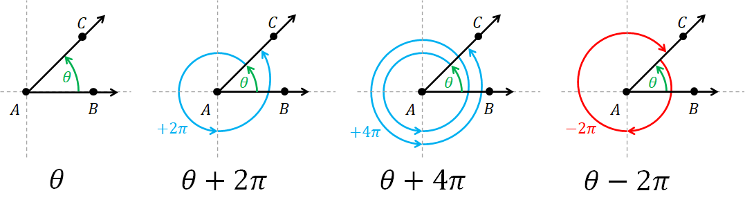
We see that the angle $\theta$ is equivalent to any angles of the form $\theta + 2\pi k$ where $k$ in an arbitrary integer, positive or negative. Symbolically, $$ \theta \equiv \theta + 2\pi k,\quad k = 0, \pm 1, \pm 2, \dotsc.$$ This is in the sense that, despite the different amount of turning one has to do, the pencil tip would end up at the same place.
3.3 Trigonometric functions
We will encounter trigonometric functions so many times later in this book because they are indispensible in doing calculation about shapes and manipulating them. We will use only three functions sine, cosine, and tangent. Let us recall what they mean.
3.3.1 Definitions based on the unit circle
Trigonometric functions are functions of an angle $\theta$, which is given to us by the functions' user. To define them, we will construct a geometric figure that depends on $\theta$ and read some information from it. The steps to construct such a figure goes as follows.
- Let $O$, $X$, and $Y$ be points such that the length of the segment $\overline{OX}$ and $\overline{OY}$ are $1$, and the signed angle $\angle(\overrightarrow{OX}, \overrightarrow{OY})$ is the positive right angle ($\pi/2$ radians or, equivalently, $90^\circ$).
- Take a compass and adjust it so that the needle point and the pencel tip are exactly 1 unit apart.
- Place the needle point on $O$ and the pencil tip on $X$.
- Turn the compass by exactly $\theta$ radians, taking the sign into account. After this is done, let the pencip tip be at point $A$.
- Draw the line segment $\overline{OA}$.
- From point $A$, draw a line segment to a point $A_X$ on the line $\overleftrightarrow{OX}$ such that $\overline{OA_X}$ is perpendicular to the line $\overleftrightarrow{OX}$. (In other words, the $\angle(\overrightarrow{OA_Y}, \overrightarrow{A_Y A})$ is $\pm 90^\circ$.)
- From point $A$, draw a line segment to a point $A_Y$ on the line $\overleftrightarrow{OY}$ such that the $\overline{OA_Y}$ is perpendicular to $\overleftrightarrow{OY}$.
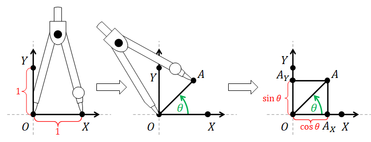
We typically call the line $\overleftrightarrow{OX}$ the $x$-axis and the line $\overleftrightarrow{OY}$ the $y$-axis. The segment $\overline{OA_X}$ and $\overline{OA_Y}$ are called the projections of $\overline{OA}$ onto the line $\overleftrightarrow{OX}$ and $\overleftrightarrow{OY}$, respectively. Let $OA_X$ and $OA_Y$ (without the lines over them) denote the length of $\overline{OA_X}$ and $\overline{OA_Y}$. We define the trigonometric functions as follows. $$ \begin{align*} \sin \theta &= \begin{cases} OA_Y, & A_Y\ \mathrm{is\ above\ } \overleftrightarrow{OX}\\ 0, & A_Y\ \mathrm{is\ on}\ \overleftrightarrow{OX}\\ -OA_Y, & A_Y\ \mathrm{is\ below\ } \overleftrightarrow{OX} \end{cases} \\ \cos \theta &= \begin{cases} OA_X, & A_X\ \mathrm{is\ to\ the\ right\ of\ } \overleftrightarrow{OY}\\ 0, & A_X \mathrm{is\ on}\ \overleftrightarrow{OY} \\ -OA_X, & A_X\ \mathrm{is\ to\ the\ left\ of\ } \overleftrightarrow{OY} \end{cases} \\ \tan\theta &= \frac{\sin \theta}{\cos \theta}. \end{align*} $$
In other words, given $\theta$, we construct a line segment of length $1$ by turning a compass starting from the $x$-axis by $\theta$ radians. After this is done, we define $\sin\theta$ to be the *signed length* of the projection of the segment onto the $y$-axis, $\cos \theta$ to be the signed length of the projection onto the $x$-axis. Lastly, $\tan \theta$ is the ratio of "$y$-projection" to the "$x$-projection." Note that $\tan \theta$ is undefined when $\cos \theta = 0$.
3.3.2 Definitions based on right triangles
The definitions above are very general and allow us to deal with negative angles and those that are outside the $[0,2\pi)$ range. However, the reader might already be familiar with the definitions that use right triangles, which goes as follows. Let $A$ be a right triangle where the angle at $A$ is $\theta$ radians, and the angle at $B$ is a right angle. The side $\overline{AB}$ is called the adjacent side to $A$, the side $\overline{BC}$ is called the opposite side to $A$, and the side $\overline{AC}$ is called the hypothenuse. Then, the triangometric functions on $\theta$ can be the defined as the following ratios of lengths.
$$ \begin{align*} \sin\theta &= \frac{BC}{AC} = \frac{\mathrm{opposite}}{\mathrm{hypothenuse}}, \\ \cos\theta &= \frac{BC}{AC} = \frac{\mathrm{adjacent}}{\mathrm{hypothenuse}}, \\ \tan\theta &= \frac{BC}{AB} = \frac{\mathrm{opposite}}{\mathrm{adjacent}}. \\ \end{align*} $$
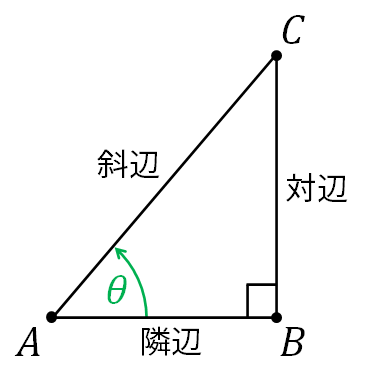
These definitions are equivalent to the ones we discussed before, but they only work when the angle at $A$ is acute (i.e., $0 \leq \theta \leq \pi/2$). This is because, without a coordinate system, we do not have a notion of negative length.
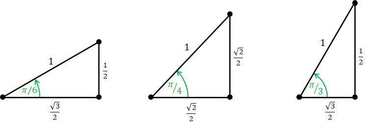
3.3.3 Example values
Let us see the values of the trigonometric functions at some well-known angles. $$ \begin{align*} \sin 0 &= 0, & \cos 0 &= 1, & \tan 0 &= 0, \\ \sin \frac{\pi}{2} &= 1, & \cos \frac{\pi}{2} &= 0, & \tan \frac{\pi}{2} &= \mathrm{undefined}, \\ \sin \pi &= 0, & \cos \pi &= -1, & \tan \pi &= 0, \\ \sin \frac{3\pi}{2} &= -1, & \cos \frac{3\pi}{2} &= 0, & \tan \frac{3\pi}{2} &= \mathrm{undefined}, \\ \sin \frac{\pi}{4} &= \frac{\sqrt{2}}{2}, & \cos \frac{\pi}{4} &= \frac{\sqrt{2}}{2}, & \tan \frac{\pi}{4} &= 1, \\ \sin \frac{\pi}{3} &= \frac{\sqrt{3}}{2}, & \cos \frac{\pi}{3} &= \frac{1}{2}, & \tan \frac{\pi}{3} &= \sqrt{3}, \\ \sin \frac{\pi}{6} &= \frac{1}{2}, & \cos \frac{\pi}{6} &= \frac{\sqrt{3}}{2}, & \tan \frac{\pi}{3} &= \frac{1}{\sqrt{3}}. \end{align*} $$
3.3.4 Some properties of trigonometric functions
We now mention some useful facts about trigonometric functions.
Equivalent angles. Recall that the angle $\theta$ is equivalent to $\theta + 2\pi k$ where $k$ is any integer because the pencil tip of the compass (i.e., the point $A$) would end up at the same place after a rotation by $\theta$ radians and $\theta + 2\pi k$ radians. As a result, $$ \begin{align*} \sin \theta &= \sin(\theta + 2\pi k),\\ \cos\theta &= \cos(\theta + 2\pi k),\\ \tan \theta &=\tan(\theta + 2\pi k). \end{align*} $$
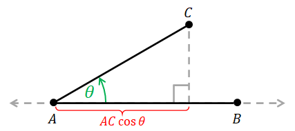
Length of projection. Next, consider two line segments $\overline{AB}$ and $\overline{AC}$ such that the angle $\angle(\overrightarrow{AB}, \overrightarrow{AC})$ is $\theta$ radians. Then, the signed length of the projection of $\overline{AC}$ onto the line $\overleftrightarrow{AB}$ is given by $$ \mathrm{signed\ length\ of\ projection} = AC \times \cos \theta. $$
Height and area of a triangle. When we want to calculate the area of the triangle $ABC$, we need to find the length of its base and its height. The length of the base is just $AB$. The height is the length of the perpendicular line from $C$ to the line $\overleftrightarrow{AB}$. We know from the definition of $\sin\theta$ That $$ \mathrm{signed\ length\ of\ perpendicular\ line} = AC \times \sin \theta. $$ As a result, $$ \mathrm{area\ of\ }ABC = \frac{1}{2} \times AB \times AC \times |\sin \theta|. $$ We take the absolute value of $\sin \theta$ because area cannot be negative. (Rest assured, though, we will talk about signed area later.)
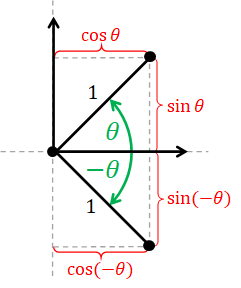
Negatives of angles. Lastly, by thinking about the relationship between points resulted from rotating the compass by $\theta$ and $-\theta$ radians, we can derive the following identities. $$ \begin{align*} \sin (-\theta) &= -\sin\theta, \\ \cos (-\theta) &= \cos\theta, \\ \tan (-\theta) &= -\tan\theta. \end{align*} $$
3.4 Vectors
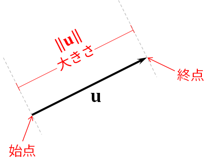
3DCG relies on linear algebra, and a fundamental concept of linear algebra is the vector. A vector is an object that has a size and a direction. In contrast, a scalar is an object that only has a size. In this book, a scalar is always a real number, and a vector is line segment between two points with an arrow indicating which way it is pointing. The point where the arrow is pointing away from is called the initial point, and the point where the arrow is pointing to is called the terminal point. We often denote a vector with bold small letters such as $\mathbf{a}$, $\mathbf{b}$, $\mathbf{c}$, $\mathbf{u}$, $\mathbf{v}$, $\mathbf{w}$, $\mathbf{x}$, $\mathbf{y}$, $\mathbf{z}$. The size of the vector is the length of the line segment, and we will use the mostly use the word "length" and "magnitude" interchangably with "size." The size (or length or magnitude) of vector $\mathbf{u}$ is denoted by $\| \mathbf{u} \|$.
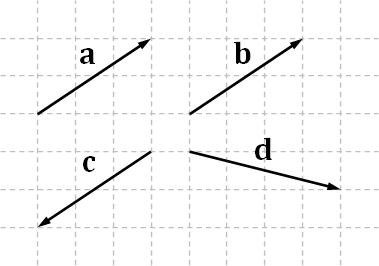
Vector equality. Basic geometric concepts such as points and line segments have definite positions. We do not treat points or lines that are at difffent places in in Euclidean space as the same entities. However, we often think of vectors as free floating in space. Two vectors are consider equal if they have the same length and point in the same direction. It doesn't matter how where the endpoints of the vectors are located.
Zero vector. There's a special vector where the initial vector and the terminal vector is the same point. This vector has length $0$ and so is called the zero vector. It is denoted by the symbol $\mathbf{0}$. Unlike other vectors, it is impossible to tell what direction the zero vector is pointing to, so its direction is undefined.
3.5 Vector arithmetic
Like numbers, we can perform calculation on vectors. Vectors admit 4 main mathematical operations, and we will discuss them in turn.
3.5.1 Scaling
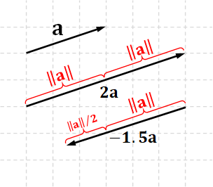
Scaling is the multiplication of a vector by a scalar, which is a real number in our case. The product of a non-zero vector $\mathbf{u}$ with a real number $a$ is denoted by $a\mathbf{u}$ is defined as follows:
- If $a = 0$, then $a\mathbf{u} = \mathbf{0}$.
- If $a > 0$, then $a\mathbf{u}$ is the vector that points in the same direction as $\mathbf{u}$ but has length $a \| \mathbf{u} \|$.
- If $a < 0$, then $a\mathbf{u}$ is the vector that points in the exact opposite direction as $\mathbf{u}$ but has length $a \| \mathbf{u} \|$.
For the zero vector, we define $a\mathbf{0} = \mathbf{0}$ for all real number $a$.
Scaling and length. Scaling is an operation that changes the vector's length. However, the direction is only gauranteed to be the same only when the scalar is positive. When the scalar is negative, the vector flips its direction. Moreover, when the scalar is zero, the direction becomes undefined. The relationship between the length of a scaled vector and the original one is given by $$ \| a\mathbf{u} \| = |a| \| \mathbf{u} \|. $$
Unit vectors. We will often work with vectors that have length $1$, and such a vector is called a unit vector. A unit vector is convenient because they can be used as yard sticks to measure distance along a direction. We sometimes signify that a vector is a unit vector by putting a hat on top of it; for examples, $\hat{\mathbf{u}}$, $\hat{\mathbf{v}}$, and $\hat{\mathbf{w}}$. Given a non-zero vector $\mathbf{u}$, we can turn it into a unit vector $\hat{\mathbf{u}}$ that points in the same direction by scaling $\mathbf{u}$ with $1/\|\mathbf{u}\|$. In other words, $$ \hat{\mathbf{u}} = \frac{\mathbf{u}}{\| \mathbf{u} \|}. $$ The process of turning a vector into a unit vector is called normalization. We thus say that unit vectors are normalized vectors, and other vectors are unnormalized. Note that the zero vector cannot be normalized at all because doing so involves division by zero.
Properties of scaling. Scaling has a number of useful properties, and we state them here without proof. First, for any real numbers $a$, $b$ and any vector $\mathbf{u}$, we have that $$ (ab) \mathbf{u} = a(b\mathbf{u}).$$ Second, $$ \mathrm{if\ }a\mathbf{u} = \mathbf{0}, \mathrm{\ then\ }a = 0\mathrm{\ or\ } \mathbf{u} = \mathbf{0}. $$ Note that the second property is very similar to a familiar property of real numbers.
Negatives of vectors. Given any vector $\mathbf{u}$, the negative of $\mathbf{u}$, denoted by $-\mathbf{u}$, is the Vector $$ -\mathbf{u} = (-1) \mathbf{u}. $$ It is the vector with has the same length as $\mathbf{u}$ but points in the exact opposite direction of $\mathbf{u}$. It should be clear that $$-(-\mathbf{u}) = \mathbf{u}.$$
3.5.2 Addition
Given two vectors $\mathbf{u}$ and $\mathbf{v}$, we can add them and produce a new vector as follows. First, we move $\mathbf{v}$ so that the initial point of $\mathbf{v}$ coincide with the terminal point of $\mathbf{u}$. Then, the sum $\mathbf{u} + \mathbf{v}$ is the vector from the initial point of $\mathbf{u}$ to the terminal point of $\mathbf{v}$.
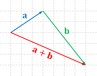
Vector addition has a nice interpretation in terms of movement. Here, we can interpret a vector as a movement in a certain direction by a certain distance. Adding two vectors results in a vector that represents executing the movement of the first vector and then executing that of the second.
Properties of addition. Vector addition has some important properties that we will not prove. First, it is commutative and associative. $$ \begin{align*} \mathbf{u} + \mathbf{v} &= \mathbf{v} + \mathbf{u}, \ (\mathbf{u} + \mathbf{v}) + \mathbf{w} &= \mathbf{u} + (\mathbf{v} + \mathbf{w}). \end{align*} $$ Second, it is distributive in conjuction with multiplication with scalars. $$ \begin{align*} (a + b)\mathbf{u} &= a\mathbf{u} + b\mathbf{u}, \ a(\mathbf{u} + \mathbf{v}) &= a\mathbf{u} + a \mathbf{v}. \end{align*} $$ Commutativity, associativity, and distributivity together allow us to manipulate vectors in pretty much the same way as we manipulate real numbers as long as we do not multiply or divide two of them.
Additive identity and inverse. Another important fact about addition is that the zero vector is the additive identity, meaning that $$ \mathbf{u} + \mathbf{0} = \mathbf{0} + \mathbf{u} = \mathbf{u} $$ for all vector $\mathbf{u}$. In particular, we have that $$ \begin{align*} \mathbf{u} + (-\mathbf{u}) = \mathbf{u} + (-1)\mathbf{u} = (1-1)\mathbf{u} = 0\mathbf{u} = \mathbf{0} \end{align*} $$ for any vector $\mathbf{u}$. Because of this, $-\mathbf{u}$ is called the additive inverse of $\mathbf{u}$ because, when added to $\mathbf{u}$, the result is the additive identity.
Additive identity and inverse. Another important fact about addition is that the zero vector is the additive identity, meaning that $$ \mathbf{u} + \mathbf{0} = \mathbf{0} + \mathbf{u} = \mathbf{u} $$ for all vector $\mathbf{u}$. In particular, we have that $$ \begin{align*} \mathbf{u} + (-\mathbf{u}) = \mathbf{u} + (-1)\mathbf{u} = (1-1)\mathbf{u} = 0\mathbf{u} = \mathbf{0} \end{align*} $$ for any vector $\mathbf{u}$. Because of this, $-\mathbf{u}$ is called the additive inverse of $\mathbf{u}$ because, when added to $\mathbf{u}$, the result is the additive identity.
3.5.3 Dot product
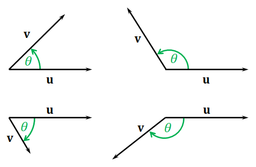
There is only one standard way to multiply two real numbers together. However, for vectors, there are two. The first way is called the dot product or the inner product, and it takes in two vectors and produces a scalar. Given two vectors $\mathbf{u}$ and $\mathbf{v}$, we first move them around so that their initial points are at the same position. Then, we measure the signed angle from $\mathbf{u}$ to $\mathbf{v}$, and let the angle be denote by $\theta$.
The dot product of $\mathbf{u}$ and $\mathbf{v}$, denoted by $\mathbf{u} \cdot \mathbf{v}$ is given by $$ \begin{align*} \mathbf{u} \cdot \mathbf{v} &= \| \mathbf{u} \| \times \| \mathbf{v} \| \times \cos\theta \\ &= (\mathrm{length\ of\ }\mathbf{u}) \times (\mathrm{signed\ length\ of\ projection\ of\ }\mathbf{v}\mathrm{\ onto\ }\mathbf{u}). \end{align*} $$
Properties of the dot product. Note that, if we swap $\mathbf{u}$ and $\mathbf{v}$, we will have that the angle from $\mathbf{v}$ to $\mathbf{u}$ is $-\theta$. So, $$ \begin{align*} \mathbf{v} \cdot \mathbf{u} &= (\mathrm{length\ of\ }\mathbf{v}) \times (\mathrm{signed\ length\ of\ projection\ of\ }\mathbf{u}\mathrm{\ onto\ }\mathbf{v}) \\ &= \| \mathbf{u} \| \times \| \mathbf{v} \| \times \cos(-\theta) \\ &= \| \mathbf{u} \| \times \| \mathbf{v} \| \times \cos \theta \\ &= \mathbf{u} \cdot \mathbf{v}. \end{align*} $$ As a result, the dot product is commutative: $$\mathbf{u} \cdot \mathbf{v} = \mathbf{v} \cdot \mathbf{u}.$$ We can also show that the following properties are true $$ \begin{align*} a(\mathbf{u} \cdot \mathbf{v}) &= (a\mathbf{u})\cdot \mathbf{v} = \mathbf{u}\cdot (a\mathbf{v}), \\ \mathbf{u} \cdot (\mathbf{v} + \mathbf{w}) &= \mathbf{u} \cdot \mathbf{v} + \mathbf{u} \cdot \mathbf{w} \end{align*} $$ for any vectors $\mathbf{u}$, $\mathbf{v}$ and any real number $a$.
Dot product and length. Because a vector always make an angle of $0$ radian with itself, we have that $$ \mathbf{u} \cdot \mathbf{u} = \| \mathbf{u} \| \times \| \mathbf{u} \| \times \cos 0 = \| \mathbf{u} \|^2. $$ In other words, $$ \| \mathbf{u} \| = \sqrt{\mathbf{u} \cdot \mathbf{u}}. $$ This formula is very important because it allows us to calculate the length of a vector very easily when we have a way to compute dot products without measuring angles. This is the case when we have a coordinate system, but it is the subject of the next chapter.
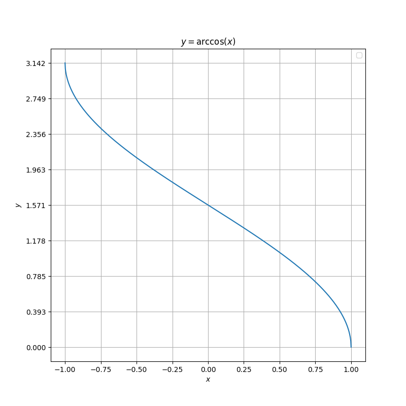
Angle in terms of dot products. From the definition of the dot product, we have that $$ \begin{align*} \cos \theta = \frac{\mathbf{u} \cdot \mathbf{v}}{\| \mathbf{u} \| \| \mathbf{v} \|} = \frac{\mathbf{u} \cdot \mathbf{v}}{\sqrt{(\mathbf{u} \cdot \mathbf{u}) (\mathbf{v} \cdot \mathbf{v})}}. \end{align*} $$ However, the value of $\theta$ that satisfies the above equation is not unique. That is, if $\theta$ satisfies it, then so do $-\theta$, $\theta + 2\pi k$, and $-\theta + 2\pi k$ for any integer $k$ because $\cos\theta = \cos(-\theta) = \cos(\theta + 2\pi k) = \cos(-\theta + 2\pi k)$. A way to avoid ambiguity is to restrict the angle to be in the range $[0, \pi]$. In this case, we can write $$ \begin{align*} \theta = \pm \arccos\bigg( \frac{\mathbf{u} \cdot \mathbf{v}}{\sqrt{(\mathbf{u} \cdot \mathbf{u}) (\mathbf{v} \cdot \mathbf{v})}} \bigg). \end{align*} $$ Here, $\arccos$ is an inverse function of $\cos$ whose range of outputs is $[0,\pi]$. In other words, if $\theta \in [0,\pi]$, we have that $\arccos$ satisfies the following property: $$ \arccos (\cos \theta) = \theta. $$
Signed length of projection. Revisiting the definition of the dot product again, we have that $$ \mathrm{signed\ length\ of\ projection\ of\ }\mathbf{v}\mathrm{\ onto\ }\mathbf{u} = \frac{\mathbf{u} \cdot \mathbf{v}}{\| \mathbf{u} \|} = \frac{\mathbf{u} \cdot \mathbf{v}}{\sqrt{\mathbf{u} \cdot \mathbf{u}}}. $$ The calculation becomes much easier if $\mathbf{u}$ is a unit vector $\hat{\mathbf{u}}$, in which case, the expression simplies to $$ \mathrm{signed\ length\ of\ projection\ of\ }\mathbf{v}\mathrm{\ onto\ }\hat{\mathbf{u}} = \frac{\hat{\mathbf{u}} \cdot \mathbf{v}}{\| \hat{\mathbf{u} \|}} = \hat{\mathbf{u}} \cdot \mathbf{v}. $$
Perpendicular vectors. We say that two vectors are perpendicular or orthogonal to each other if the angles between them is a right angle; that is, any angle of the form $\pm \pi/2 + 2\pi k$ for any integer $k$. When $\mathbf{u}$ and $\mathbf{v}$ are perpendicular, it follows that $$ \begin{align*} \mathbf{u} \cdot \mathbf{v} = \| \mathbf{u} \| \times \| \mathbf{v} \| \times \cos \bigg(\pm \frac{\pi}{2} + 2\pi k \bigg) = \| \mathbf{u} \| \times \| \mathbf{v} \| \times 0 = 0. \end{align*} $$ Hence, checking whether the dot product between two vectors is zero or not is a convenient way to see if they are perpendicular to each other or not.
Notationally, we write $\mathbf{u} \perp \mathbf{v}$ to denote the fact that the two vectors are perpendicular to each other.
Paralllel vectors. We say that two vectors are parallel to each other if they point in the same direction or exactly in the opposite direction. Another way to say this is that, if $\theta$ is the angle between the two vectors, then $\theta$ is equivalent to $0$ radians (pointing in the same direction) or $\pi$ radians (pointing in the opposite directions). This implies that $\cos\theta = \pm 1$, and it follows that $$ \mathbf{u} \cdot \mathbf{v} = \| \mathbf{u} \| \| \mathbf{v} \| \cos\theta = \pm \| \mathbf{u} \| \| \mathbf{v} \|. $$ In other words, $$ |\mathbf{u} \cdot \mathbf{v}| = \| \mathbf{u} \| \| \mathbf{v} \|. $$ Notationally, we write $\mathbf{u} \parallel \mathbf{v}$ to denote the fact that the two vectors are perpendicular to each other.
Vector decomponsition. Given two vectors $\mathbf{u}$ and $\mathbf{v}$ with $\mathbf{u} \neq \mathbf{0}$, we can write $\mathbf{v}$ as a sum of two vectors $$\mathbf{v} = \mathbf{v}_\parallel + \mathbf{v}_\perp$$ where (1) $\mathbf{v}_\parallel$ is parallel to $\mathbf{u}$, and (2) $\mathbf{v}_\perp$ is perpendicular to $\mathbf{u}$.
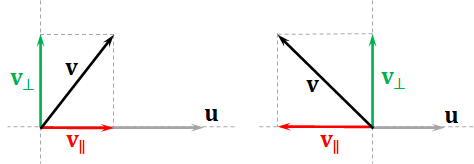
The parallel component is just the projection of $\mathbf{v}$ onto the line through $\mathbf{u}$. $$ \begin{align*} \mathbf{v}_\parallel &= (\mathrm{signed\ length\ of\ projection\ of\ }\mathbf{v}\mathrm{\ onto\ }\mathbf{u}) \times (\mathrm{unit\ vector\ that\ points\ in\ the\ direction\ of\ \mathbf{u}}) \\ &= \frac{\mathbf{u} \cdot \mathbf{v}}{\| \mathbf{u} \|} \frac{\mathbf{u}}{\| \mathbf{u} \|} \\ &= \frac{\mathbf{u} \cdot \mathbf{v}}{\| \mathbf{u} \|^2} \mathbf{u}. \end{align*} $$ The perpendicular component can then be obtained by subtracting the parallel component from $\mathbf{v}$. $$ \mathbf{v}_\perp = \mathbf{v} - \mathbf{v}_\parallel = \mathbf{v} - \frac{\mathbf{u} \cdot \mathbf{v}}{\| \mathbf{u} \|^2} \mathbf{u}. $$ As a sanity check, we can see if $\mathbf{v}_\perp$ is really perpendicular to $\mathbf{u}$ by seeing if their dot product is zero. This is actually the case because $$ \begin{align*} \mathbf{u} \cdot \mathbf{v}_\perp &= \mathbf{u} \cdot \bigg( \mathbf{v} - \frac{\mathbf{u} \cdot \mathbf{v}}{\| \mathbf{u} \|^2} \mathbf{u} \bigg) = \mathbf{u} \cdot \mathbf{v} - \frac{\mathbf{u} \cdot \mathbf{v}}{\| \mathbf{u} \|^2} (\mathbf{u} \cdot \mathbf{u}) = \mathbf{u} \cdot \mathbf{v} - \frac{\mathbf{u} \cdot \mathbf{v}}{\| \mathbf{u} \|^2} \| \mathbf{u} \|^2 = \mathbf{u} \cdot \mathbf{v} - \mathbf{u} \cdot \mathbf{v} = 0. \end{align*} $$
3.5.4 Cross product
The cross product is another standard way to multiply to vectors together. It is different from other operations because it is only defined on three-dimensional vectors while other operations also work on two-dimensonal vectors (or vectors in higher-dimensional spaces) too.
Given two 3D vectors $\mathbf{u}$ and $\mathbf{v}$, the cross product of $\mathbf{u}$ and $\mathbf{v}$, denoted by $\mathbf{u} \times \mathbf{v}$, is another vector in 3D space. For simplicity, let us assume that both $\mathbf{u}$ and $\mathbf{v}$ are non-zero first. To compute the cross product, we move $\mathbf{u}$ and $\mathbf{v}$ so that their initial points coincide. We then form a quadriliteral from the following 4 points:
- $A$ = the initial point of $\mathbf{u}$ and $\mathbf{v}$,
- $B$ = the terminal point of $\mathbf{u}$,
- $C$ = the terminal point of $\mathbf{u} + \mathbf{v}$, and
- $D$ = the terminal point of $\mathbf{v}$.
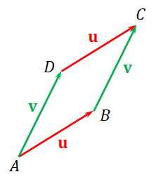
We then compute the area of $ABCD$, which is equal to $$ \begin{align*} 2 \times (\mathrm{area\ of\ triangle\ }ABC) = 2 \times \frac{1}{2} \times AB \times BC \times |\sin \theta| = \| \mathbf{u} \|\, \| \mathbf{v} \|\, |\sin \theta| \end{align*} $$ where $\theta$ is the angle from $\mathbf{u}$ to $\mathbf{v}$. The length of the cross product is this area. In other words, $$ \begin{align*} \| \mathbf{u} \times \mathbf{v} \| = \| \mathbf{u} \|\, \| \mathbf{v} \|\, |\sin \theta|. \end{align*} $$
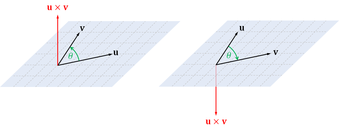
The direction that the cross product points is rather complicated to describe. The cross product is required to be perpendicular to both $\mathbf{u}$ and $\mathbf{v}$. As a result, it is also perpendicular to the plane that contains them and the quadriliteral $ABCD$. However, for any 2D plane in a 3D space, there are two directions that are perpendicular to the plane as can be seen in the figure below. In other words, the plane containing $\mathbf{u}$ and $\mathbf{v}$ splits the 3D space into two "half-spaces," and the cross product points towards one of them.
We decide which half-space the cross product would point towards based on the sign of the angle $\theta$ determined from our point of view. As an observer in 3D, we look at the plane from a half-space.
- If, from our point of view, the angle $\theta$ is positive (i.e., it takes a counterclockwise rotation to get from $\mathbf{u}$ to $\mathbf{v}$), then $\mathbf{u} \times \mathbf{v}$ should point to the half-space that we, the observer, are in. In other words, it should point towards us.
- On the hand, if $\theta$ is negative (i.e., it takes a clockwise rotation to get from $\mathbf{u}$ to $\mathbf{v}$), then $\mathbf{u} \times \mathbf{v}$ should point to the half-space that we are not in. It should point away from us. The above two rules are consistent. The direction of the cross product would be the same no matter which side the observer is in.
One way to remember the above rule is to use a mnemonic called the right-hand rule. With your right hand, stick your thumbs out so that it is perpendicular to the direction of your index finger. Now, arrange your hand in 3D so that the rotation you see when you curl your index finger towards the palm agrees with the rotation to get from $\mathbf{u}$ to $\mathbf{v}$. Then, the cross product $\mathbf{u} \times \mathbf{v}$ should point in the direction of your thumb.
We have just defined the cross product when $\mathbf{u}$ and $\mathbf{v}$ are non-zero. The case for when at least when of the vectors is zero is simple, we just define $\mathbf{u} \times \mathbf{v}$ to be the zero vector.
Properties of the cross product. The cross product is associative. $$ \begin{align*} (\mathbf{u} \times \mathbf{v}) \times \mathbf{w} = \mathbf{u} \times (\mathbf{v} \times \mathbf{w}). \end{align*} $$ However, it is not commutative because $$ \begin{align*} \mathbf{u} \times \mathbf{v} = - (\mathbf{v} \times \mathbf{u}). \end{align*} $$ Because the angle a vector makes with itself is $0$ radian, we have that $$ \begin{align*} \| \mathbf{u} \times \mathbf{u} \| = \| \mathbf{u} \|^2 \sin 0 = 0. \end{align*} $$ As a result, $$\mathbf{u} \times \mathbf{u} = \mathbf{0}.$$ Like the dot product, the cross product is distributive with respect to vector addition. $$ \begin{align*} \mathbf{u} \times (\mathbf{v} + \mathbf{w}) &= (\mathbf{u} \times \mathbf{v}) + (\mathbf{u} \times \mathbf{v}) \\ (\mathbf{u} + \mathbf{v}) \times \mathbf{w} &= (\mathbf{u} \times \mathbf{w}) + (\mathbf{v} \times \mathbf{w}). \end{align*} $$ Lastly, scalar multiplication goes through the cross product. That is, $$ (c\mathbf{u}) \times \mathbf{v} = c(\mathbf{u} \times \mathbf{v}) = \mathbf{u} \times (c\mathbf{v}). $$
3.6 Point arithmetic
As discussed earlier, a vector is a quantity that has a magnitude and a direction. On the other hand, a point is a position in space, having neither magnitude nor direction. Some arithmetic operations can be performed on points, but these are much more restrictive than what we can do with a vector.
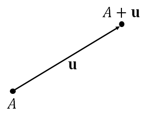
Point-vector addition. We can add a vector $\mathbf{u}$ to a point $A$. To do so, move $\mathbf{u}$ so that its initial point coincides with $A$. The sum is the point that is the position of the terminal point of $\mathbf{u}$.
Subtraction. We also can subtract a point $A$ from another point $B$. The result, $B - A$, is a vector whose initial point is $A$ and terminal point is $B$. In other words, $B - A$ is the displacement from $A$ to $B$.
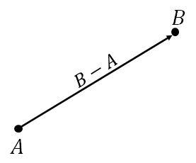
We can see that point subtraction is the reverse operation of adding a vector to a point. In other words, if $\mathbf{u} = B - A$, we have that $B = A + \mathbf{u}$, which leads to the following identity: $$ A + (B - A) = B,$$ which makes sense arithematically.
One consequence of defining point subtraction this way is that it allows us to write the area of a triangle in terms of the points that makes up the triangle. In other words, if $A$, $B$, and $C$ are three points that form a triangle, we can let $\mathbf{u} = B - A$ and $\mathbf{v} = C - A$. From our earlier discussion on the length of $\mathbf{u} \times \mathbf{v}$, we know that it is equal to two times the area of the triangle that is created from (1) the initial points of $\mathbf{u}$ and $\mathbf{v}$, (2) the terminal point of $\mathbf{u}$, and (3) the terminal point of $\mathbf{v}$. These points are $A$, $B$, and $C$, respectively. As a result, we have that $$ \mathrm{area\ of\ }\triangle ABC = \frac{1}{2} \big\| (B-A) \times (C-A) \big\|. $$
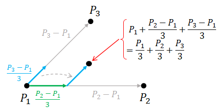
Linear combination of points. Given $n$ points $P_1$, $P_2$, $\dotsc$, $P_n$, a linear combination of points is an expression of the form $$ c_1 P_1 + c_2 P_2 + \dotsb + c_n P_n $$ where $c_1$, $c_2$, $\dotsc$, $c_n$ are real numbers. Not all linear combinations result in a point, only those such that $$c_1 + c_2 + \dotsb + c_n = 1$$ are allowed. When this condition is satisfied, the linear combination is defined to be the point $$ c_1 P_1 + c_2 P_2 + \dotsb + c_n P_n = P_1 + c_2(P_2 - P_1) + c_3(P_3 - P_1) + \dotsb + c_n(P_n - P_1). $$ Note that the quantity on the RHS is a point. This is because (1) $P_i - P_1$ is a vector, (2) $c_i(P_i - P_1)$ is also a vector, and (3) each of the vector is added to the point $P_1$, which would result in a point. Note also that we have not defined any mathematical operations that are employed on the LHS at all. We have not defined how to multiply a point with a scalar, and we have not defined how to add such products together. We are simply saying that, when the coefficients add up to one, the scaled points can be added together to yield a point. Otherwise, the answer is undefined and should not be used.
3.7 Using point and vector arithmetic to define shapes
A point of studying vectors, points, and their mathematical operations is that we can use it to define shapes of virtual objects that we would put in our virtual scenes. We have been discussing shapes such as triangles and circles before, but we have not really defined what they exactly are. This makes it hard to process them with a computer. So, in this section, we will revisit many of the geometric shapes we have been taken for granted and formally define them. A shape is a set of points that satisfy some conditions, and we can specify these conditions using the arithmetic operations we have learned so far.
3.7.1 Circles and spheres
Perhaps the easiest shapes to define with point and vector arithmetic are a circle and a sphere. Their definitions are the same. The only difference is that a circle is two-dimensional, but a sphere is three-dimensional. To make the discussion succinct, let us only discuss the sphere. To define one, we need a point $O$ (the center) and a real number $r < 0$ (the radius). A sphere a set of all points that is at distance $r$ from $O$. In other words, if $P$ is a point on the sphere, the vector $P - O$ must have length $r$. That is, $$ \begin{align*} \mathrm{sphere\ of\ radius\ } r \mathrm{\ with\ center\ } O = \{ P : \| P - O \| = r \}. \end{align*} $$
3.7.2 Straigh lines, rays, and line segments
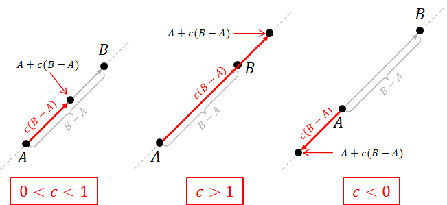
Given two points $A$ and $B$ which are not the same, consider the expression $$ \begin{align*} A + c(B - A). \end{align*} $$ We see that $B - A$ is a vector that is pointing in the direction from $A$ to $B$. So, adding a scaled version $c(B - A)$ to $A$ results in a point on the straight line $\overleftrightarrow{AB}$. In particular,
- when $c = 0$, we have that $A + c(B - A) = A$,
- when $c = 1$, we have that $A + c(B - A) = A + (B - A) = B$,
- when $0 < c < 1$, we have that $A + c(B - A)$ lies between $A$ and $B$,
- when $c > 1$, we have that $A + c(B - A)$ is further away from $A$ than $B$, and
- when $c < 0$, we have that $A + c(B - A)$ is "behind" $A$ in the opposite direction of $B - A$.
As a result, we can equate the straight line $\overleftrightarrow{AB}$, the line $\overrightarrow{AB}$, and the line segment $\overline{AB}$ as: $$ \begin{align*} \overleftrightarrow{AB} &= \{ A + c(B-A) : c \in \mathbb{R} \},\\ \overleftarrow{AB} &= \{ A + c(B-A) : c \geq 0 \}, \\ \overline{AB} &= \{ A + c(B-A) : 0 \leq c \leq 1 \}. \\ \end{align*} $$
3.7.3 Planes
Given three points $A$, $B$, and $C$ that are distinct and do not lie on the same straight line. (That is, they are not collinear.) We have that the vectors $B - A$ and $C - A$ are non parellel to one other because, if they are, the three points would lie on a single straight line.
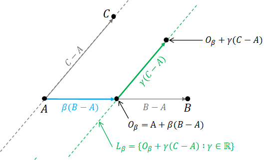
Consider an expression of the form $$ A + \beta(B-A) + \gamma(C - A) $$ where $\beta$ and $\gamma$ are real numbers. Let $O_\beta$ denote $A + \beta(B - A)$. We know that $O_\beta$ is a point on the straight line $\overleftrightarrow{AB}$. Now, consider the set $$ L_\beta = \{ O_\beta + \gamma (C - A) : \gamma \in \mathbb{R} \}. $$ We have that it is a straight line that is parallel to $\overleftrightarrow{AC}$ that passes through $O_\beta$.
Now, if we let $\beta$ take any real value and collect all the set $L_\beta$ together, we have that all these set of lines would form the plane that the points $A$, $B$, and $C$ resides in.
As a result, $$ \begin{align*} \mathrm{plane\ of\ }A, B, C = \{ A + \beta(B - A) + \gamma(C - A) : \beta, \gamma \in \mathbb{R} \}. \end{align*} $$ Note that we learned earlier that $A + \beta(B - A) + \gamma(C - A)$ can be rewritten as $$ \alpha A + \beta B + \gamma C $$ where $\alpha + \beta + \gamma = 1$. (That is, just set $\alpha = 1 - \beta - \gamma$.) Hence, we have another way to define a plane. $$ \begin{align*} \mathrm{plane\ of\ }A, B, C = \{ \alpha A + \beta B + \gamma C : \alpha, \beta, \gamma \in \mathbb{R} \mathrm{\ and \ } \alpha + \beta + \gamma = 1 \} \end{align*} $$ Consequently, a plane containing three non-collinear points is the set of all linear combinations of the three points such that the coefficients add up to one.
3.7.4 Barycentric coordinates
Based on the definition above, we have that, for any point $P$ on the plane defined by point $A$, $B$, and $C$, there would be a unique combination of real numbers $\alpha$, $\beta$, and $\gamma$ such that $$ P = \alpha A + \beta B + \gamma C, \quad \mathrm{and} \quad \alpha + \beta + \gamma = 1.$$ The real numbers $\alpha$, $\beta$, and $\gamma$ are called the **barycentric coordinates** of point $P$. Let us examine the meaning of each coefficient. Consider $\beta$. From the reasoning in the last section, the set of all points on the plane with $\beta$ fixed to a real value is the set $$ \begin{align*} L_\beta = \{ O_\beta + \gamma(C - A) : \gamma \in \mathbb{R} \} \end{align*} $$ where $O_\beta = A + \beta(B - A)$. It is a straight line that is parallel to the straightline $\overleftrightarrow{AC}$. We have that the following are true.
- When $\beta = 0$, it follows that $O_\beta = A$, and the line passes through $A$ and $C$.
- When $\beta = 1$, it follows that $O_\beta = B$, and the line passes through $B$.
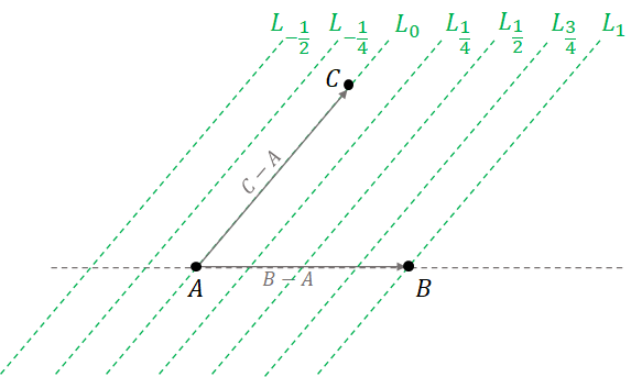
- When $\beta = 0.5$, it follows that $O_\beta$ is half way between $A$ and $B$, so the line is also half way between $\overleftrightarrow{AC}$ and $B$.
The lines $L_\beta$ for other values of $\beta$ are drawn in Figure 3.26.
In general, the coefficient $\beta$ of point $P$ can be interpreted as the distance between $P$ and the straight line $\overleftrightarrow{AC}$ in a unit such that the point $B$ is at distance $1$. A way to express this interpretation is to say $$ \begin{align*} \beta = \frac{\mathrm{signed\ distance\ between\ } P \mathrm{\ and\ } \overleftrightarrow{AC}}{\mathrm{distance\ between\ } B \mathrm{\ and\ } \overleftrightarrow{AC}}. \end{align*} $$ Note that the nominator is a signed distance because, if $P$ were to be not on the same side of $\overleftrightarrow{AC}$ as $B$, the distance would be negative.
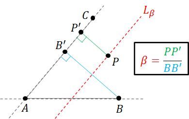
Now, we can multiply both the nominator and the denominator by the length of $\overline{AC}$ and $1/2$. We have that $$ \begin{align*} \beta &= \frac{(\mathrm{signed\ distance\ between\ } P \mathrm{\ and\ } \overleftrightarrow{AC}) (\mathrm{length\ of\ } \overline{AC})/2}{(\mathrm{distance\ between\ } B \mathrm{\ and\ } \overleftrightarrow{AC}) (\mathrm{length\ of\ } \overline{AC})/2} \\ &= \frac{\mathrm{signed\ area\ of\ }\triangle APC}{\mathrm{area\ of\ }\triangle ABC} \\ &= \pm \frac{\mathrm{area\ of\ }\triangle APC}{\mathrm{area\ of\ }\triangle ABC} \end{align*} $$ where the sign of $\beta$ is positive if $P$ is on the same side of $\overleftrightarrow{AC}$ as $B$ and negative otherwise.
There is yet another way to interpret $\beta$. Recall from the section on point subtraction that we can write the area of a triangle in terms of the length of a cross product. It follows that $$ \begin{align*} \beta &= \pm \frac{\mathrm{area\ of\ }\triangle APC}{\mathrm{area\ of\ }\triangle ABC} = \pm \frac{\big\| (C - A) \times (P - A)\big\|/2}{\big\|(C - A) \times (B - A)\big\|/2} &= \pm \frac{\big\|(C - A) \times (P - A)\big\|}{\big\|(C - A) \times (B - A)\big\|}. \end{align*} $$ The above formula allows us to compute $\beta$ by measuring the length of $C-A$, $P-A$, and $B-A$ and the angles between some of them.
We have discussed at length about the meaning of $\beta$. However, there is nothing special about $\beta$ because we can apply the same reasoning to $\alpha$ and $\gamma$. It follows, then, that the barycentric coordinate $(\alpha, \beta, \gamma)$ of a point $P$ on the plane defined by the three points satisfy the following properties: $$ \begin{align*} \alpha &= \frac{\mathrm{signed\ distance\ between\ } P \mathrm{\ and\ } \overleftrightarrow{BC}}{\mathrm{distance\ between\ } A \mathrm{\ and\ } \overleftrightarrow{BC}} = \pm \frac{\mathrm{area\ of\ }\triangle PBC}{\mathrm{area\ of\ }\triangle ABC} = \pm \frac{\big\|(B - C) \times (P - C)\big\|}{\big\|(B - C) \times (A - C)\big\|}, \\ \beta &= \frac{\mathrm{signed\ distance\ between\ } P \mathrm{\ and\ } \overleftrightarrow{AC}}{\mathrm{distance\ between\ } B \mathrm{\ and\ } \overleftrightarrow{AC}} = \pm \frac{\mathrm{area\ of\ }\triangle APC}{\mathrm{area\ of\ }\triangle ABC} = \pm \frac{\big\|(C - A) \times (P - A)\big\|}{\big\|(C - A) \times (B - A)\big\|}, \\ \gamma &= \frac{\mathrm{signed\ distance\ between\ } P \mathrm{\ and\ } \overleftrightarrow{AB}}{\mathrm{distance\ between\ } C \mathrm{\ and\ } \overleftrightarrow{AB}} = \pm \frac{\mathrm{area\ of\ }\triangle ABP}{\mathrm{area\ of\ }\triangle ABC} = \pm \frac{\big\|(A - B) \times (P - B)\big\|}{\big\|(A - B) \times (C - B)\big\|}. \end{align*} $$
3.7.5 Another definition of a plane
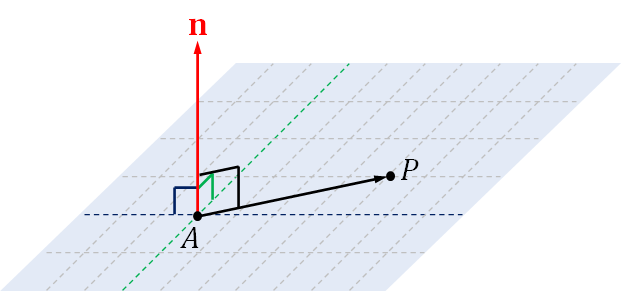
There's another way to define the plane we have been discussing so far. Because $B-A$ and $C-A$ are non-zero and are not parallel, their cross product $$ \mathbf{n} = (B - A) \times (C-A) $$ is a non-zero vector that is perpendicular to both $B-A$ and $C-A$. In particular, if $P$ is a point on the plane containing $A$, $B$, and $C$, then we would be able to find its barycentric coordinates $(\alpha, \beta, \gamma)$ such that $$ \begin{align*} P &= \alpha A + \beta B + \gamma C \\ &= A + \beta(B - A) + \gamma(C - A). \end{align*} $$ So, we have that $$ \begin{align*} \mathbf{n} \cdot (P - A) &= \mathbf{n} \cdot \big[ \beta(B - A) + \gamma(C - A) \big] \\ &= \mathbf{n} \cdot \big[ \beta(B - A)\big] + \mathbf{n} \cdot \big[\gamma(C - A) \big] \\ &= \beta \big[ \mathbf{n} \cdot (B - A)\big] + \gamma \big[ \mathbf{n} \cdot (C - A)\big] \\ &= \beta(0) + \gamma(0) \\ &= 0. \end{align*} $$ Thus, $\mathbf{n}$ is perpendicular to $P-A$ for any point $P$ in the plane. Hence, another way to define a plane is to write $$ \begin{align*} \mathrm{plane\ of\ }A, B, C = \{ P : \mathbf{n} \cdot (P - A) = 0 \mathrm{\ and\ } \mathbf{n} = (B - A) \times (C - A) \}. \end{align*} $$ In a sense, the vector $\mathbf{n}$ or any vector that is parallel to it is perpendicular to the whole plane, and so it is called a normal vector to the plane.
In fact, we can define a plane by specifying a point $A$ and a normal vector $\mathbf{n}$ instead of specifying three points. The definition becomes $$ \begin{align*} \mathrm{plane\ containing\ }A\mathrm{\ and\ perpendicular\ to\ }\mathbf{n} = \{ P : \mathbf{n} \cdot (P - A ) = 0 \}. \end{align*} $$
3.7.6 Triangles
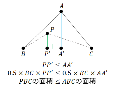
Like a plane, a triangle is also defined by three points $A$, $B$, and $C$ that do not lie on a straight line. Because the triangle defined these points is a part of the plane defined by the same points, each point $P$ in the triangle can be written as $$\alpha A + \beta B + \gamma C $$ where the coefficients of the points are their barycentric coordinates. However, because the triangle does not include as many points as the plane, there needs to be extra constraints on the coordinates, and the constraints are: $$ \begin{align*} 0 \leq \alpha \leq 1,\\ 0 \leq \beta \leq 1,\\ 0 \leq \gamma \leq 1. \end{align*} $$ To see why the above conditions must hold, consider the coordinate $\alpha$. First, if $\alpha < 0$, then $P$ would be on the opposite side of $\overleftrightarrow{BC}$ than $A$ and so would be outside of the triangle $ABC$. Hence, $\alpha$ must be at least $0$. Second, it must also be the case that $\alpha \leq 1$ because, if $P$ is in the triangle $ABC$, then the area of the triangle $PBC$ must be not greater than the area of the triangle $ABC$. As a result, $$ \alpha = \frac{\mathrm{area\ of\ }\triangle PBC}{\mathrm{area\ of\ }\triangle ABC} \leq 1. $$
Note that the same reasoning can also be done to $\beta$ and $\gamma$. As a result, we have that the triangle $ABC$ is defined as follows: $$ \triangle ABC = \{ \alpha A + \beta B + \gamma C : 0 \leq \alpha, \beta, \gamma \leq 1 \mathrm{\ and\ } \alpha + \beta + \gamma = 1 \}. $$ Recall that an expression of the form $\alpha A + \beta B + \gamma C$ is called a linear combination. A linear combination where the coefficients are non-negative and add up to one is called a convex combination. Thus, the triangle $ABC$ is the set of convex combinations of $A$, $B$, and $C$.
3.8 Summary
- Computer graphics makes heavy use of geometry to define shapes of virtual objects.
- A shape is a set of points in Euclidean space. One can define a shape by writing conditions that the points in it have to satisfy.
- Conditions on points can be written in terms of arithmetic of points and vectors.
- A point represents a position. It has no magnitude.
- A vector has magnitude and a direction. Generally, it denotes the movement to get to one point from another (i.e., the operation of point subtraction).
- A point is fixed in space, but a vector can move around freely.
- We can add and subtract vectors and multiply them with scalars. There are no restrictions on these operations.
- However, while we can subtract one point from another, multiplying a point with a scalar and adding points together are not generally defined. We can only do so when the coefficients of the points add up to $1$.
- Important shapes include
- circles and spheres: $$ \mathrm{circle\ or\ sphere\ of\ radius\ } r \mathrm{\ with\ center\ } O = \{ P : \| P - O \| = r \}, $$
- straight lines, rays, line segments: $$ \begin{align*} \overleftrightarrow{AB} &= \{ A + c(B-A) : c \in \mathbb{R} \},\\ \overleftarrow{AB} &= \{ A + c(B-A) : c \geq 0 \}, \\ \overline{AB} &= \{ A + c(B-A) : 0 \leq c \leq 1 \}, \\ \end{align*} $$
- planes: $$ \begin{align*} \mathrm{plane\ containing\ points\ } A, B, C &= \{ \alpha A + \beta B + \gamma C : \alpha, \beta, \gamma \in \mathbb{R}\mathrm{\ and\ } \alpha + \beta + \gamma = 1\}, \\ \mathrm{plane\ containing\ } A \mathrm{\ with\ normal\ vector\ }\mathbf{n} &= \{ P : \mathbf{n} \cdot (P - A) = 0 \}, \end{align*} $$
- triangles $$ \triangle ABC = \{ \alpha A + \beta B + \gamma C : \alpha A + \beta B + \gamma C : 0 \leq \alpha, \beta, \gamma \leq 1 \mathrm{\ and\ } \alpha + \beta + \gamma = 1 \}.$$
- A point $P$ in a plane defined by three non-collinear points $A$, $B$, $C$ can be written as a linear combination $\alpha A + \beta B + \gamma C$ where $\alpha + \beta + \gamma = 1$. The tuple $(\alpha, \beta, \gamma)$ is called the barycentric coordinate of $P$, and they satisfy the following equations. $$ \begin{align*} \alpha &= \frac{\mathrm{signed\ distance\ between\ } P \mathrm{\ and\ } \overleftrightarrow{BC}}{\mathrm{distance\ between\ } A \mathrm{\ and\ } \overleftrightarrow{BC}} = \pm \frac{\mathrm{area\ of\ }\triangle PBC}{\mathrm{area\ of\ }\triangle ABC} = \pm \frac{\big\|(B - C) \times (P - C)\big\|}{\big\|(B - C) \times (A - C)\big\|}, \\ \beta &= \frac{\mathrm{signed\ distance\ between\ } P \mathrm{\ and\ } \overleftrightarrow{AC}}{\mathrm{distance\ between\ } B \mathrm{\ and\ } \overleftrightarrow{AC}} = \pm \frac{\mathrm{area\ of\ }\triangle APC}{\mathrm{area\ of\ }\triangle ABC} = \pm \frac{\big\|(C - A) \times (P - A)\big\|}{\big\|(C - A) \times (B - A)\big\|}, \\ \gamma &= \frac{\mathrm{signed\ distance\ between\ } P \mathrm{\ and\ } \overleftrightarrow{AB}}{\mathrm{distance\ between\ } C \mathrm{\ and\ } \overleftrightarrow{AB}} = \pm \frac{\mathrm{area\ of\ }\triangle ABP}{\mathrm{area\ of\ }\triangle ABC} = \pm \frac{\big\|(A - B) \times (P - B)\big\|}{\big\|(A - B) \times (C - B)\big\|}. \end{align*} $$