5 Modeling with meshes
In the last chapter, we introduced a way to represent simple geometric concepts such as points, vectors, lines, and circles with numbers. In this chapters, we will discuss how these simple geometric concepts can be combined to build more complex shapes that can be used to build scenes in computer graphics applications.
We note first that there are many ways to represent shapes with numbers, but we shall focus on one particular method: modeling with meshes. This is the method used by the graphics pipeline, the rendering algorithm implemented in modern GPUs. We choose the method because this book is mainly about teaching you how use WebGL, a software library that control GPUs to draw 3D shapes in real time.
To drop a few names, other methods include point clouds, splines, distance fields, and volumetric data. We will not cover them in this book, but curious readers can consult other computer graphics textbooks to learn more about them.
5.1 Vertices
The graphics pipeline is designed to render three types of simple geometric concepts: points, line segments, and triangles. More complex shapes such as circles, ellipses, chairs, human figures, and so on must be built from these objects in order to be rendered by the graphics pipeline.
The three geometric concepts have one thing in common: they can be specified by points.
- A point is already a point.
- A line segment can be specified by its two endpoints.
- A triangle can be specified by its three corners, all of which are points.
In computer graphics, a point used to defined a shape is called a vertex. A vertex can have one or more attributes, which is a fancy term for data associated with the point. Simply put, a vertex is a point that carries some data with it.
The most important and mandatory attribute of a vertex is its position in 3D space. We know from the previous chapter that a position can be represented by 3 floating-point numbers.
Other widely used attributes include:
- color,
- normal vector, and
- texture coordinates.
We know from Chapter 2 that a color can be represented by three numbers: $R$, $G$, and $B$. We will discuss what a normal vector in Chapter 6, but, since it is a vector in 3D space, it can be represented by their coordinates, which are 3 numbers. Texture coordinates will be discussed in Chapter 18?, but they can be represented by 2 numbers most of the time.
More concretely, we can discuss a vertex in terms of the Javascript language, which we will be programming with. A vertex can be thought of as a Javascript object. Its attributes can be thought of the object's (Javascript) properties. As an example, here is a vertex written in the JSON format.
{
    "position": [1.0, 2.0, 3.0],
    "normal": [0.0, 1.0, 0.0],
    "color": [1.0, 0.0, 1.0],
    "texCoord": [0.5, 0.5]
}
5.2 Point clouds
We said that, in order to use the graphics pipeline to render complex shapes, we must model them with simple shapes, which in turn can be constructed from vertices. So, a shape to be rendered by the graphics pipeline must be made from a collection of vertices. A collection of related vertices is often called a point cloud.
Typically, all data of a point cloud is stored in one or more arrays of numbers, where each such array is called a buffer. In general, there are two ways to organize vertex data into buffers.
- Interleaved buffer. Use a single buffer to store all vertex attributes together, grouping attributes of the same vertex together.
- Separate buffers. Put each attribute into its own separate buffer. In this way, a point cloud is a collection of buffers, which can include the position buffer, color buffer, normal buffer, texture coordinate buffer, and so on.
To illustrate the above data layouts, let us consider a small point cloud with 3 vertices, each having a position attribute, and a texture coordinate attribute.
| Vertex Number | #0 | #1 | #2 |
| Position | $(0.0, 0.1, 0.2)$ | $(1.0, 1.1, 1.2)$ | $(2.0, 2.1, 2.2)$ |
| Texture coordinate | $(0.50, 0.51)$ | $(0.60, 0.61)$ | $(0.70, 0.71)$ |
If we were to construct an interleaved buffer of the above point cloud, the buffer look like the following.
| 0.0 | 0.1 | 0.1 | 0.51 | 0.52 | 1.0 | 1.1 | 1.1 | 0.61 | 0.62 | 2.0 | 2.1 | 2.2 | 0.71 | 0.72 |
In the Javascript language, this would be equivalent to specifying the following array.
const interleavedBuffer = [
    0.0, 0.1, 0.2,  // Vertex #0's position
    0.50, 0.51,     // Vertex #0's texture coordinate
    1.0, 1.1, 1.2,  // Vertex #1's position
    0.60, 0.61,     // Vertex #1's texture coordinate
    2.0, 2.1, 2.2,  // Vertex #2's position
    0.70, 0.71      // Vertex #2's texture coordinate
];
On the other hand, if we were to create separate buffers for the point cloud. We would have the following two buffers.
| Position: |
|
|||||||||
| Texture coordinate: |
|
|||||||||
In the Javascript language, the above is equivalent to the following code.
const positionBuffer = [
    0.0, 0.1, 0.2,  // Vertex #0's position
    1.0, 1.1, 1.2,  // Vertex #1's position
    2.0, 2.1, 2.2,  // Vertex #2's position
];

const texCoordBuffer = [
    0.50, 0.51,     // Vertex #0's texture coordinate
    0.60, 0.61,     // Vertex #1's texture coordinate
    0.70, 0.71      // Vertex #2's texture coordinate
];
In the context of the graphics pipeline, a point cloud alone is not enough to represent shapes. However, we also said earlier that a point cloud can represent shape on its own. This approach is not at all trivial because we immediately see a problem: a point cloud has no contiguous surface or volume that we typically associate with real world objects. In other words, the space between the points are empty, and the empty space would manifest if we look at the object from a distance close enough. As a result, any method that uses point clouds alone to represent shapes must come up with a way to fill these "holes." In any case, this is not our problem because we will use point clouds with extra information.
5.3 Primitives
The extra information that helps us fill the empty space between vertices are how to "group" or "connect" vertices so that they form simple geometric shapes. A shape specified by connecting vertices is called a primitive.
Different implementations of the graphics pipeline have different primitives they support. In general, though, the primitives are some forms of points, lines, or triangles. WebGL, the implementation that we will use, supports the following primitives.
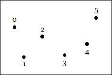
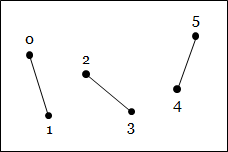
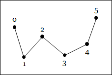
- Point. Specified by a single vertex.
- Line. Specified by two vertices, which serve as its endpoints.
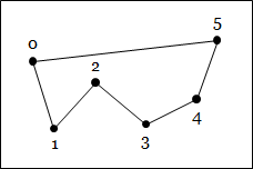
- Line strip. Specified by an arbitrary number of vertices in a list. The primitive is a collection of line segments connecting consecutive vertices.
- Line loop. Also specified by an arbitrary number of vertices in a list. This primitive is just a line strip primitive with an extra line segment connecting the first and the last vertex together.
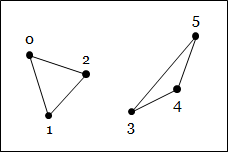
- Triangle. Specified by three vertices, which serve as its corners.
- Traingle strip. Specified by an arbitrary number of vertices in a list. This primitive is a set of connected triangles. The first three vertices from the first triangle. For each new vertex in the list, a new triangle is formed between itself and the two vertices that come before it.
- Triangle fan. Specified by an arbitrary number of vertices in a list. Again, this primitive is a collection of connected triangles, and the first triangle is formed from the first three vertices. For each new vertex, a new triangle is formed between itself, the vertex that comes before it, and the first vertex. The primitive can thus be thought of as a "fan" that emanates from the first vertex.
 |
|||
| Points | |||
 |
 |
 |
|
| Lines | Line strip | Line loop | |
 |
 |
 |
|
| Triangles | Triangle strip | Triangle fan |
Internally, WebGL uses integer constants to indicate primitive types. Each constant also has a namethat can be used to retrieve them more conveniently in Javascript programs, and we will make use of these names extensively in later chapters. The constants and their names are given in the table below.
| Primitive | Constant Value | Constant Name |
| Points | 0 | POINTS |
| Lines | 1 | LINES |
| Line loop | 2 | LINE_LOOP |
| Line strip | 3 | LINE_STRIP |
| Triangles | 4 | TRIANGLES |
| Triangle strip | 5 | TRIANGLE_STRIP |
| Triangle fan | 6 | TRIANGLE_FAN |
5.4 Meshes
In WebGL, shapes are modeled by meshes. A mesh is a point cloud together with information about how to connect the vertices to form primitives. A mesh can contain many primitives, but in general all the primitives would be of the same type. So, we may have a triangle mesh or a wireframe (a mesh of line segments). Meshes of other primitives are possible, but they are not as frequently used as the two we just mentioned.
If we were to represent a mesh as a Javascript object, the object would contain three important pieces of data.
- The type of primitives in the mesh.
- A buffer or multiple buffers containing attributes of vertices in the point cloud.
- Another buffer called the index buffers that contains the indices of vertices in the point cloud that should be connected to form primitives.
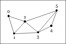
5.4.1 An example triangle mesh
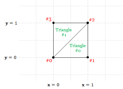
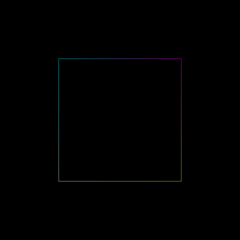
Below is a mesh representing a $1 \times 1$ square in the $xy$-plane whose lower-left endpoint is the origin $(0,0,0)$.
const TRIANGLES  = 4;

const mesh = {
    "primitive": TRIANGLES,
    "positions": [
        0.0, 0.0, 0.0,  // Vertex #0's position
        1.0, 0.0, 0.0,  // Vertex #1's position
        1.0, 1.0, 0.0,  // Vertex #2's position
        0.0, 1.0, 0.0   // Vertex #3's position
    ],
    "colors": [
        1.0, 1.0, 1.0,  // Vertex #0's color (white)
        1.0, 1.0, 0.0,  // Vertex #1's color (yellow)
        1.0, 0.0, 1.0,  // Vertex #2's color (magenta)
        0.0, 1.0, 1.0   // Vertex #3's color (cyan)
    ],
    "indices": [
        0, 1, 2,  // Triangle #0
        0, 2, 3   // Triangle #1
    ]
};
 |
 |
We see that there are 4 vertices in the mesh. Each vertex has two attributes, its position and color. The vertices are used to form two triangles, and a triangle is represented by 3 consecutive indices in the index buffer, resulting in 6 numbers in total. An advantage of this representation is that the data of a vertex can be used multiple times (Vertex 1 and Vertex 2 are used 2 times), saving space.
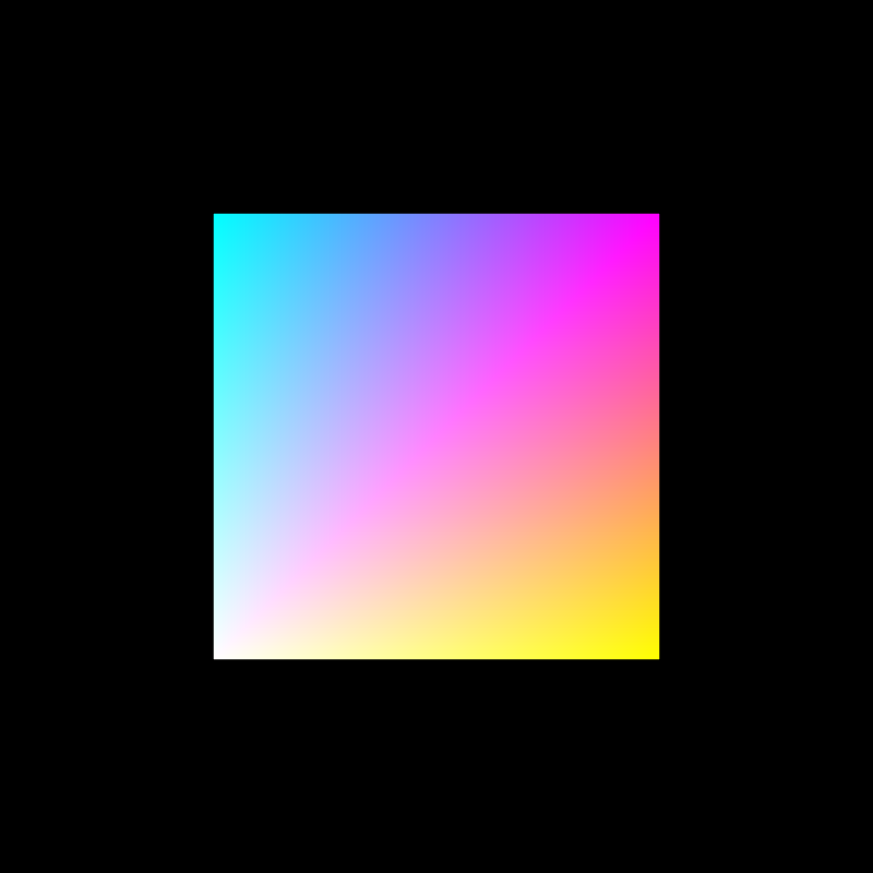
When rendering a mesh, we, the programmer, can control how WebGL deals with the vertex attributes by writing small programs called "shaders," and we will talk about them in details in later chapters. The program that generated the rendering in Figure 5.4 did the most basic processing: simply outputting the specified colors. Note that we only specified 4 colors (white, yellow, magneta, and cyan) at the corners, but we see many more colors (or shades of them) in the rendering. This is because, when WebGL renders a triangle, it must decide what colors the pixels that are between the vertices should have, and the typical behavior is to interpolate between the colors of the corner vertices. As a result, the colors of pixels that belong to Triangle #0 (the bottom right one) are combinations of white (Vertex #0's color), yellow (Vertex #1's color) and magneta (Vertex #2's color). On the other hand, the colors of Triangle #1's pixels are combinations of white, magenta, and cyan.
5.4.2 An example wireframe
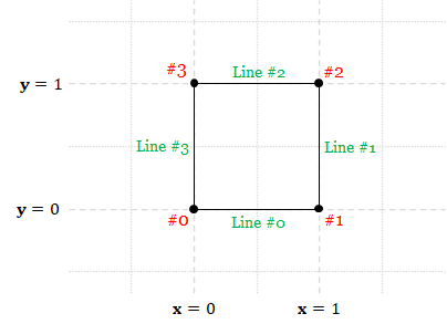
The following is a wireframe created from the same point cloud as the triangle mesh in the last section.
const LINES = 1;

const mesh = {
    "primitive": LINES,
    "positions": [
        0.0, 0.0, 0.0,  // Vertex #0's position
        1.0, 0.0, 0.0,  // Vertex #1's position
        1.0, 1.0, 0.0,  // Vertex #2's position
        0.0, 1.0, 0.0   // Vertex #3's position
    ],
    "colors": [
        1.0, 1.0, 1.0,  // Vertex #0's color (white)
        1.0, 1.0, 0.0,  // Vertex #1's color (yellow)
        1.0, 0.0, 1.0,  // Vertex #2's color (magenta)
        0.0, 1.0, 1.0   // Vertex #3's color (cyan)
    ],
    "indices": [
        0, 1,  // Line #0
        1, 2,  // Line #1
        2, 3,  // Line #2
        3, 0,  // Line #3
    ]
};
 |
 |
The differences between the wireframe and the triangle mesh are (1) the primitive type and (2) the index buffer. Here, a line primitive is defined by two nsecutive indices. Because the index buffer has 8 numbers, it defines 4 lines in total. Like what we saw with the traingle mesh earlier, the pixels between the vertices have colors that are interpolations of the vertex colors.
5.5 Surface modeling with triangle meshes
Now that we understand what a mesh is, it is a good time to step back and see what it can do for us. Recall that, in order to create 3D-looking images with computer graphics, we must create a scene that is populated with objects. Meshes allow us to model these objects. However, what actually are we modeling with meshes?
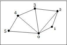
A physical object has volume that is filled with matter. Nevertheless, unless the constituent matter is translucent, we would not see what lies inside the object and would only see the matter that makes the object's surface. For example, a human is made of flesh, blood, bones, and many complicated internal organs. In normal circumstances, we only see his/her skin and externals features such as hair, eyes, nose, and so on. As a result, for most physical objects, it is wasteful to model their internal structures. Modeling only their surfaces are often enough to convey the shapes.
Accordingly, most 3D models are just surfaces: contiguous sets of points in 3D that are intrinsically two-dimensional in the sense that they have no thickness. Such a surface and be closed, meaning that they partition the space into two regions: the "inside" and "outside." Because the inside of a real-world object is often invisible, the inside of most 3D models are just hollow to save memory and modeling efforts. (See Figure 5.6.) Most solid objects—an apple, a chair, a rock, etc.—can be modeled with as closed surfaces. If a surface is not closed, we say that it is open. We often model thin objects such as a piece of paper or a ribbon with open surfaces.
 |
 |
 |
| (a) | (b) | (c) |
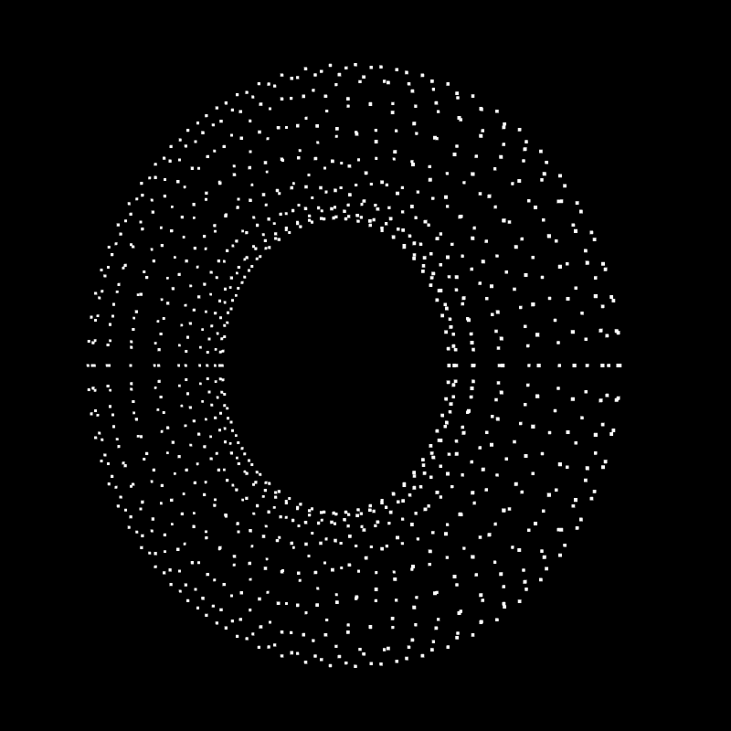
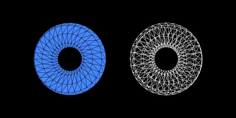
In most real-time computer graphics applications, surfaces are modeled by triangle meshes. A triangle on its own is a very simple surface, but a triangle mesh—effectively a collection of multiple triangles—can represent much more complex surfaces. A triangle has only 3 corners and 3 edges. However, by arranging triangles so that their edges coincide, we can make polygons with more sides and corners like the square in Figure 5.4. A triangle is always flat and open, but multiple triangles can be connected to form a closed surface that looks curved like the torus in Figure 5.3. In fact, any complex surfaces can be approximated to a high degree of accuracy by using enough small triangles.
Representing surfaces with triangle meshes has an obvious limitation. Because a triangle is flat, a triangle mesh is also flat when looked at from a distance close enough. This means that a curved surface like a sphere or a torus cannot be represented absolutely correctly by triangle meshes.
 |
 |
 |
| (a) | (b) | (c) |
5.6 Summary
- The graphics pipline can only render simple shapes such as points, line segments, and triangles. As a result, we must model shapes of more complicated objects from these simple shapes.
- The simple shapes are created by connecting points together. A point used to create a simple shape is called a vertex.
- A vertex can have attributes, which are data associated with it. Common attributes include:
- position,
- color,
- normal vector, and
- texture coordinates.
- A collection of related vertices is called a point cloud.
- A primitive is a shape specified by connecting vertices together.
- WebGL, the implemention of the graphics pipeline we shall study in this book, support 6 types of primitives, which include points, line segments, and triangles.
- A mesh is a point cloud together with information aoout how the vertices are connected to form primitives.
- A mesh typically has only one type of primitives. The most common types of meshes are:
- triangle meshes, and
- wireframes, which are meshes of line segments.
- We model shapes of objects by modeling only their external surfaces because we often cannot see an object's internal structure.
- Triangle meshes can be used to model very complex surfaces. More details can be added by using smaller triangles and more of them.
- Triangles are flat. As a result, triangle meshes cannot model curved surfaces absolutely correctly because they would appear flat when looked at from a distance close enough.